
Fibre Foam Conductivity
Quick Start
The basics of fibre foams are no different from those of conventional Foam Conductivity, they just look a bit different when you plot them in the same way.
Credits
We use papers from a team in U Colorado and Xi’an Jiaotong U12
Fibre Foam Conductivity
//One universal basic required here to get things going once loaded
window.onload = function () {
    //restoreDefaultValues(); //Un-comment this if you want to start with defaults
    Main();
};

//Main() is hard wired as THE place to start calculating when inputs change
//It does no calculations itself, it merely sets them up, sends off variables, gets results and, if necessary, plots them.
function Main() {
    //Save settings every time you calculate, so they're always ready on a reload
    saveSettings();

    //Send all the inputs as a structured object
    //If you need to convert to, say, SI units, do it here!
    const inputs = {
        Kgas: sliders.SlideKgas.value, //keep in mW
        rhorel: sliders.Sliderhorel.value,
        Ksolid: sliders.SlideKsolid.value, //keep in mW
        kabs: sliders.Slidekabs.value * 100, //to m-1
        dgas: sliders.Slidedgas.value*1e-12, //from pm to m
        dFibre: sliders.SlidedFibre.value/1e6, //from um to m
        T: sliders.SlideT.value + 273, //to K
        rhoSolid: sliders.SliderhoSolid.value,
        LinearPlot: document.getElementById('LinearPlot').checked,
    };

    //Send inputs off to CalcIt where the names are instantly available
    //Get all the resonses as an object, result


    const result = CalcIt(inputs);

    //Set all the text box outputs
   // document.getElementById('phiStrut').value = result.phiStrut;
    document.getElementById('rhoFoam').value = result.rhoFoam;
   // document.getElementById('Solid').value = result.sInfo;
    //Do all relevant plots by calling plotIt - if there's no plot, nothing happens
    //plotIt is part of the app infrastructure in app.new.js
    if (result.plots) {
        for (let i = 0; i < result.plots.length; i++) {
            plotIt(result.plots[i], result.canvas[i]);
        }
    }

    //You might have some other stuff to do here, but for most apps that's it for Main!
}

//Here's the app calculation
//The inputs are just the names provided - their order in the curly brackets is unimportant!
//By convention the input values are provided with the correct units within Main
function CalcIt({ Kgas,Ksolid,kabs,dgas,dFibre,rhoSolid, rhorel, T,LinearPlot }) {
    const Kscorr=Ksolid*(0.2060*T + 115.5811)/(0.2060*298 + 115.5811)
    Kgas*=(0.07411*T + 3.40294)/(0.07411*298 + 3.40294)
    //const n=1+0.4*rhorel
    const n=1+0.4*rhorel
    const kB=1.38e-23,SB=5.67e-8,xsi=1.64,ri2=n*n
    const P=100000 //Not bothering with variable T and P input
    const Lambda=kB*T/(1.414*Math.PI*dgas*dgas*P)
    let Kabs=kabs*rhorel
    //The constant from PU foam is too small to simulate fibres, so it's halved from 1.82 to 0.91
    const KN1=1.82E-02,	KN2=0.771646381,KN3=0.006352564,KN4=2121.269214
    //Output real foam density
    let rhoFoam=rhorel*rhoSolid

    //Strut calcs in μm from Glicksman
    //const Lv=8.6/(phiCell*phiCell)
    //const a=Math.sqrt(fs*rhorel/(0.29*Lv))
    //const phiStrut=Math.sqrt(4*0.29/Math.PI*a*a)
    const dFum=dFibre*1e6
    let phium=2*dFibre*1e6, inc=1,phi=0,Kn=0,Kg=0,Kr=0,Kt,N=0,KoverN=0,Kscat=0,HiTerm=0, Ksg=0
    let pKs=[],pKg=[],pKr=[],pKt=[],pRel=[],phinm=0,porosity=0, thePorosity=0
    let minrrDiff=99999,rrDiff=0, phiumrel=0, Ktmax=0
    while (phium <= 1000){ //um steps for convenience
        phi=phium/1e6
        phinm=phium*1000
        porosity=(phi**3+3*dFibre*phi**2)/(phi+dFibre)**3
        rhorelnow=(1-porosity)
        rrDiff=Math.abs(rhorel-rhorelnow)
        if (rrDiff < minrrDiff){
            minrrDiff = rrDiff
            phiumrel=phium
            thePorosity=porosity
        }
        Kabs=kabs*rhorelnow
        if (phi > 2* dFibre && porosity > 0.8){
        Ks=Kscorr*4*(dFibre/2/(phi+dFibre))**2
        //A trivial correction for other conduction path
        Ksg=(dFibre)**2/(dFibre/Kscorr+2*phi/Kgas)/(phi+dFibre)
        Ks+=Ksg
        Kg=Kgas*(phi/(phi+dFibre))**2
        N=Math.pow(6/(Math.PI*Math.pow(phi,3))*(1-rhorelnow),0.3333)
        //The crude fitting function
        KoverN=KN1*Math.pow(phinm,KN2)*KN3*(1-Math.exp(-phinm/KN4))
        Kscat=N*KoverN
        let Kradtot=Kscat+Kabs
        //Increase from 16 to 64 as fitting
        Kr=1000*64*ri2*SB*Math.pow(T,3)/(3*Kradtot)
        Kt=Ks+Kg+Kr
        pKs.push({x:phium-dFum,y:Ks})
        pKg.push({x:phium-dFum,y:Kg})
        pKr.push({x:phium-dFum,y:Kr})
        pKt.push({x:phium-dFum,y:Kt})
        Ktmax=Math.max(Ktmax,Kt)
        }
        phium+=inc
        //if (phinm>=10*inc) inc*=10
    }
    pRel.push({x:phiumrel,y:0}) ;  pRel.push({x:phiumrel,y:Ktmax})
//Now set up all the graphing data.
//We use the amazing Open Source Chart.js, https://www.chartjs.org/
//A lot of the sophistication is addressed directly here
//But if you need something more, read the Chart.js documentation or search Stack Overflow
const plotData=[pKs,pKg,pKr,pKt, pRel]
const lineLabels=["Solid","Gas","Radiative","Total","Actual"]
const myColors=["gray","blue","orange","red","magenta"]

//Now set up all the graphing data detail by detail.
const prmap = {
    plotData: plotData, //An array of 1 or more datasets
    lineLabels: lineLabels, //An array of labels for each dataset
    colors: myColors, //An array of colors for each dataset
    hideLegend: false,
    borderWidth: [2, 2, 2 ,3,1],
    xLabel: 'φ&μm', //Label for the x axis, with an & to separate the units
    yLabel: 'K&mW/mK', //Label for the y axis, with an & to separate the units
    y2Label: null, //Label for the y2 axis, null if not needed
    yAxisL1R2: [], //Array to say which axis each dataset goes on. Blank=Left=1
    logX: !LinearPlot, //Is the x-axis in log form?
    xTicks: function(value, index, ticks) {if (value.toPrecision(2).includes("1") || value.toPrecision(2).includes("5")) {if (value>=1) {return value.toFixed(0)} else {return value.toPrecision(1)} } else {return ""}; },
    logY: false, //Is the y-axis in log form?
    yTicks: undefined, //We can define a tick function if we're being fancy
    legendPosition: 'top', //Where we want the legend - top, bottom, left, right
    xMinMax: [,], //Set min and max, e.g. [-10,100], leave one or both blank for auto
    yMinMax: [,], //Set min and max, e.g. [-10,100], leave one or both blank for auto
    y2MinMax: [,], //Set min and max, e.g. [-10,100], leave one or both blank for auto
    xSigFigs: 'P1', //These are the sig figs for the Tooltip readout. A wide choice!
    ySigFigs: 'F1', //F for Fixed, P for Precision, E for exponential
};

//Now we return everything - text boxes, plot and the name of the canvas, which is 'canvas' for a single plot
return {
    plots: [prmap],
    canvas: ['canvas'],
    //phiStrut: (phiStrut).toPrecision(2),
    rhoFoam: (rhoFoam).toFixed(0) + " : "+thePorosity.toFixed(3),
};
}
The basics
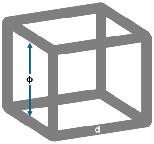 The two papers assume that the fibres are arranged as cubic cells with air spacing φ (they use D, but defined differently between their papers) and fibre thickness d.
We then have conduction by 3 routes. With some simplifications these are:
- Solid `K_s=K_"fibre"*(d/(φ+d))^2`
- Gas `K_g=K_"gas"*((φ+d)/d)^2`
- Radiation: A complex formula
The Solid and Gas corrections are simply mirror images of each other. The papers include an extra term called S-G. It's included in the app for completeness but is insignificant in practice. As starting values for simulations, Ks for cellulose fibres is ~600 and for glasswool it is ~1300 mW/m.K. Kgas is 26 for air.
Although the radiative effect has choice of two formulae, the key values are obtained by simplistic fitting so here the radiative formula from the other paper is used, tweaked to mimic the values in these two papers. There are two effects - absorption, which can be described simply, and scattering which depends on the emissivity, ε, of the fibres which, in turn, depends on their surface properties. The idea seems to be that if you can roughen the surface of the fibres, ε and radiative losses go down.
The graph
Depending on the pore size φ we see how the different conductive contributions change. The original papers use 3 different types of plot to capture the variations. However, some of those plots have unrealistic fibre and/or pore sizes, reflecting the authors' academic approach. Here we match the other app so you can control ρrel with the calculated real density shown. Because we want to specify the fibre diameter, d, we can't independently know or specify φ, so the graph shows the φ value for your current setup. If you need a specific φ you can alter the d or ρrel sliders, whichever suits you best, to get the line on your desired pore size. The relationship between φ, d and ρrel controls the porosity, ψ, which is shown in the output box. The interplay between the parameters is given by:
`ψ=(φ^3+3φ^2d)/(φ+d)^3`
`ρ_"rel"=1-ψ`
Because we use ρrel as an input, while users measure ρfoam, you need to know ρsolid which is ~1500 for cellulose and 2200 for glasswool.
The optimum fibre foam
The radiative effect falls of gradually as you increase the amount of fibre as does, of course, the gas conductivity. But the solid conductivity increases to counter those effects. At the same time you have the trade-offs between fibre diameter and pore size, with mechanical and producibility issues influencing your choice. It's complicated - that's why we have an app.
Convection
There is no convection term in the calculation because if you carry out a conventional thermal conductivity test there are zero convection effects except for theoretical foams with super-fine fibres, high porosities and large pores. Technically, for all relevant foams, the porous Rayleigh number, Ra << 40, which is when convection starts.
However, these fibre foams are notorious for showing strong convection losses in real life. A wonderfully old-fashioned and thorough paper from ORNL3 explains why. If the top surface of the foam is exposed to the atmosphere then the Rayleigh calculation becomes irrelevant and you can (and do) have large losses in insulation, especially if (e.g. in an attic roof) there is plenty of air movement. So remember that unlike a classic closed cell PU foam, fibre foams (or inorganic fibres) are unsuitable for insulation without a good surface barrier to prevent convection losses.
1He Liu and Xinpeng Zhao, Thermal Conductivity Analysis of High Porosity Structures with Open and Closed Pores, Int. J. Heat & Mass Transfer 183 (2022) 122089
2Xingrong Lian et al, Thermal conductivity analysis of natural fiber-derived porous thermal insulation materials, Int. J. Heat & Mass Transfer 220 (2024) 124941
3Agnès A. Delmas and Kenneth E. Wilkes, Numerical Analysis of Heat Transfer by Conduction and Natural Convection in Loose-Fill Fiberglass Insulation - Effects of Convection on Thermal Performance, ORNL/CON-338
