Relaxation and Creep

A spring and dashpot in series give you a Maxwell fluid which can simulate Relaxation, but not Creep. A spring and dashpot in parallel give you a Kelvin-Voigt solid which can simulate Creep but not Relaxation

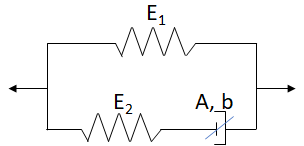
Here we use a "modified standard solid" model developed by Evagelia Kontou and others¹ which has a spring and dashpot in series plus a spring and (the same) dashpot in parallel. The key is that the parallel spring is a "strain hardening" one, with no strength at zero strain, and we use a non-linear "Eyring" dashpot.

We need 5 parameters for this (rather than the two each for Maxwell and Kelvin-Voigt). So it's important to get a feel for what each one means

1. E₁. This is the hardening spring made from two components which I've called E₁ & E₁₁, though in the literature these are called η₁ & η₂. If E₁₁=0 then we have a simple spring.
2. E₂. This is the Maxwell spring.
3. A & b. These make up the non-linear dashpot. A is the response rate or frequency, and b controls the non-linearity. When b is very small then we have a simple dashpot.

The original papers are "polymer" papers so the key values are in terms of MPa. For soft-matter rheology it makes sense to use Pa. You can switch between the two sets of units.

Recovery

One of the distinctive features of these experiments is that if the strain or stress is suddenly removed, the system starts to recover. If the strain or stress is then re-applied after a time, the original behaviour re-starts. One such cycle can be performed with strain or stress being removed at t_stop and resumed after after a delay of t_hold.

The Equations

The strain-hardening spring, using the η notation is, for strain ε:

`E_1=η_1ε^(-η_2)`

The non-linear dashpot at stress σ is given by:

`(δε)/(δt) = A"sinh"[b(σ-εE_1)]`

For a constant strain ε the Relaxation curve is given by:

`(δσ)/(δt) = -AE_2sinh[b(σ-εE_1)]`

For constant stress σ the Creep curve is given by:

`(δε)/(δt) = (AE_2sinh[b(σ-εE_1')])/[E_2+E_1(1+η_2)]` where `E_1' = η_1ε^(1-η_2)`