Shear-Dependent Viscosity

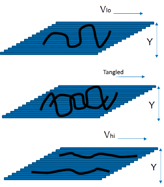We know that the simple viscosity relationship discussed in Viscosity Basics was derived by Newton and fluids which obey that law are Newtonian fluids. The cause of viscous drag is familiar to those who drive in busy traffic. If a driver in a slow lane moves into a faster lane that causes the cars behind to slow down to accommodate the new arrival. For ordinary molecules in liquids their random movement between streamlines causes the same slowing down (viscous drag). When polymer molecules are concerned, if one part of the polymer is in one streamline and another part is in a different streamline then the polymer starts to be stretched, causing a bigger drag between streamlines. The effect is larger if concentrations and MWts are large enough to create tangles. However, with faster streamlines (with V going from lo-->hi) the polymer chains tend, on average, to become more and more aligned with the flow so they cause proportionally less drag between the streamlines. So higher shear leads to lower viscosity in many polymer systems. For such non-Newtonian systems the graph of viscosity versus shear rate can be conveniently described using the Cross formula:

`η = η_"inf"+(η_0-η_"inf")/(1+(α.γ̇)^n)`

where η_inf is the viscosity at (essentially) infinite shear, η₀ is the viscosity at zero shear and α and n are fitting constants.

The same formula handles dilatant systems where the viscosity gets higher with shear. The explanation for that is a log-jam effect where particles/polymers can't respond (reorientate) quickly enough when bumping into each other.

Different Views

Most of us are used to seeing viscosity plotted versus log shear rate. It is therefore a shock to see it plotted versus linear shear rate. Rheologists prefer to plot shear stress versus shear rate (with and without logs) and this is even more of a shock. It's worth playing around with both the Cross model parameters and the different ways of looking at the same data. Finally, some rheologists prefer to plot viscosity versus stress, which changes the plot somewhat by pushing the curve to higher values. See below for the Power Law option

Different parts of your process create different shear rates and therefore different viscosities. It is easy to estimate the shear rate for any given process. Squeezing an adhesive or paint at 5cm/s from a nozzle that is 0.5cm diameter gives a shear rate of 5/0.5=10 while the same adhesive being squeezed or paint being applied as a 10μm layer at 0.1m/s gives a shear rate of 0.1/10^-5=10⁴. Enter the estimated shear rate and the relevant viscosity and shear stress are calculated.

Power Law

Although the Power Law (or Ostwald Law) curve is essentially useless (the Cross model is much more realistic and general), it remains popular so if you click the Show Power Law option you can see its effect. The equation (slightly modified to be consistent with η₀ and η_inf) is:

`η = η_"inf"+(η_0-η_"inf")γ̇^(n-1)`

The equation blows up γ̇<1 so the value is fixed at η ₀ for these values. The reason some people use the power law curve is that they can provide a single number, sometimes called "P Ostwald", to use on, say, a product data sheet.