
Capillary Suspensions
Quick Start
Capillary suspensions are a way to get a rather boring, low % suspension of particles in an incompatible fluid to become super viscous by adding a small % of another incompatible fluid.
Credits
The app is based on a paper from Ashish V. Orpe's team at CSIR in Pune which builds on the pioneering work of Koos et. al. Errors of interpretation are all mine.
Capillary Suspensions
//One universal basic required here to get things going once loaded
window.onload = function () {
    //restoreDefaultValues(); //Un-comment this if you want to start with defaults
    Main();
};

//Main() is hard wired as THE place to start calculating when inputs change
//It does no calculations itself, it merely sets them up, sends off variables, gets results and, if necessary, plots them.
function Main() {
    //Save settings every time you calculate, so they're always ready on a reload
    saveSettings();

    //Send all the inputs as a structured object
    //If you need to convert to, say, SI units, do it here!
    const inputs = {
        R: sliders.SlideR.value/1e6/2, //μm to m, D to R
        G: sliders.SlideGamma.value/1e3, //mN/m to N/m
        phip: sliders.Slidephip.value/100, //from %
        phis: sliders.Slidephis.value/100,
    };

    //Send inputs off to CalcIt where the names are instantly available
    //Get all the resonses as an object, result


    const result = CalcIt(inputs);

    //Set all the text box outputs
    document.getElementById('ty').value = result.ty;
    document.getElementById('phisp').value = result.phisp;
    //Do all relevant plots by calling plotIt - if there's no plot, nothing happens
    //plotIt is part of the app infrastructure in app.new.js
    if (result.plots) {
        for (let i = 0; i < result.plots.length; i++) {
            plotIt(result.plots[i], result.canvas[i]);
        }
    }

    //You might have some other stuff to do here, but for most apps that's it for Main!
}
const m1lim=0.8, m1cut=0.005, m2fact=0.025, Mag=20
let K=0

//Here's the app calculation
function CalcIt({R, G, phip, phis }) {
    let yconp=[],ycons=[]
    K=Mag*G/R
    const phisp=phis/phip
    const S=1-phis/(1-phip)
    const tmpty=Calcy(phis,phip)
    const ty=tmpty>999 ? tmpty.toPrecision(4):tmpty.toPrecision(3)
    let i=0, s=0, p=0, t=0
     for (i=0;i<100;i++){
        s=0.001+0.01*i/100
        t= Calcy(s,phip)
        yconp.push({x:s*100,y:t})
        p=0.05+0.3*i/100
        t=Calcy(phis,p)
        ycons.push({x:p*100,y:t})
        }

    const plotData = [yconp]
    const plotData1 = [ycons]
    const lineLabels = ["τy const φs"]
    const myColors = ["orange"]
    const borderWidth = [2, 2, 2]

    //Now set up all the graphing data detail by detail.
    const prmap = {
        plotData: plotData, //An array of 1 or more datasets
        lineLabels: ["τy const φp"], //An array of labels for each dataset
        colors: myColors, //An array of colors for each dataset
        hideLegend: false,
        borderWidth: borderWidth,
        xLabel: 'φs&%', //Label for the x axis, with an & to separate the units
        yLabel: 'τy&Pa', //Label for the y axis, with an & to separate the units
        y2Label: null, //Label for the y2 axis, null if not needed
        yAxisL1R2: [], //Array to say which axis each dataset goes on. Blank=Left=1
        logX: false, //Is the x-axis in log form?
        xTicks: undefined, //We can define a tick function if we're being fancy
        logY: false, //Is the y-axis in log form?
        yTicks: undefined, //We can define a tick function if we're being fancy
        legendPosition: 'top', //Where we want the legend - top, bottom, left, right
        xMinMax: [,], //Set min and max, e.g. [-10,100], leave one or both blank for auto
        yMinMax: [,], //Set min and max, e.g. [-10,100], leave one or both blank for auto
        y2MinMax: [,], //Set min and max, e.g. [-10,100], leave one or both blank for auto
        xSigFigs: 'P3', //These are the sig figs for the Tooltip readout. A wide choice!
        ySigFigs: 'P3', //F for Fixed, P for Precision, E for exponential
    };
    const prmap1 = {
        plotData: plotData1, //An array of 1 or more datasets
        lineLabels: ["τy const φs"], //An array of labels for each dataset
        colors: myColors, //An array of colors for each dataset
        hideLegend: false,
        borderWidth: borderWidth,
        xLabel: 'φp&%', //Label for the x axis, with an & to separate the units
        yLabel: 'τy&Pa', //Label for the y axis, with an & to separate the units
        y2Label: null, //Label for the y2 axis, null if not needed
        yAxisL1R2: [], //Array to say which axis each dataset goes on. Blank=Left=1
        logX: false, //Is the x-axis in log form?
        xTicks: undefined, //We can define a tick function if we're being fancy
        logY: false, //Is the y-axis in log form?
        yTicks: undefined, //We can define a tick function if we're being fancy
        legendPosition: 'top', //Where we want the legend - top, bottom, left, right
        xMinMax: [,], //Set min and max, e.g. [-10,100], leave one or both blank for auto
        yMinMax: [,], //Set min and max, e.g. [-10,100], leave one or both blank for auto
        y2MinMax: [,], //Set min and max, e.g. [-10,100], leave one or both blank for auto
        xSigFigs: 'P3', //These are the sig figs for the Tooltip readout. A wide choice!
        ySigFigs: 'P3', //F for Fixed, P for Precision, E for exponential
    };

    //Now we return everything - text boxes, plot and the name of the canvas, which is 'canvas' for a single plot
    return {
        plots: [prmap, prmap1],
        canvas: ['canvas', 'canvas1'],
        ty: ty,
        phisp:phisp.toPrecision(3)+" : "+S.toPrecision(3),
    };
}
function Calcy(phis,phip){
    let m1=(phis < m1cut)?m1lim*Math.pow(phis/m1cut,2):m1lim
    const m1lo=0.85,m1hi=1.2
    if (phis > m1lo*m1cut && phis < m1hi*m1cut){ //Stop the abrupt transition
        const t = (phis/m1cut-m1lo)/(m1hi-m1lo), P1=0.46, P2=0.53
        // A cubic Bezier to smooth
        m1=Math.pow(1-t,3)*m1lim*Math.pow(phis/m1cut,2)+3*Math.pow(1-t,2)*t*P1+3*(1-t)*t*t*P2+t*t**t*m1lim
   }
    const m2=phis/m2fact
    return K*m1*Math.pow(phis/m2,2)/(1/phip-2.5)
}
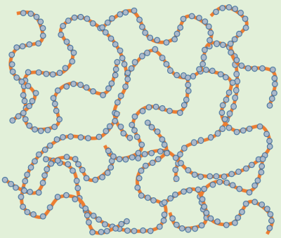 You have some particles (light blue) in an incompatible fluid (light green). They might be hydrophobic particles in water, or hydrophilic particles in oil. We know that at volume fractions, φ > 28% that you start to get some significant viscosity and yield stress, as described in the High Shear Particles app. But at a low φ of, say, 5%, nothing interesting happens.
Then you add 0.5% of a secondary fluid (orange) which, like the particle, isn't too happy in the bulk fluid - a drop of oil if you have a water suspension or a drop of water if you have an oil suspension. Suddenly the whole system becomes solid. You've just created a Capillary Suspension, where the particles are joined together via capillary bridges formed from the secondary fluid.
Many of us have encountered this phenomenon by accident and never understood it. And the basic physics has been around since the 19th century. But it was Koos & Willenbacher at KIT who properly launched the topic in 2011. Since then the field has expanded enormously as there are obviously many systems where gellation from a small fraction of particles and an even smaller fraction of secondary liquid is useful.
Although the principle is delightfully simple, the practice is tricky for a few reasons, nicely described in a recent review by Koos' team at U Leuven1 where you can find lots of references to the rest of the capillary suspension literature:
- Getting the incompatible particles into a fluid and dispersing the incompatible oil into the bulk fluid can both be tricky - usually it needs plenty of high-speed mixing.
- If you introduce lots of air in the mixing it is very hard to get it out, so you need a smart mixing setup.
- If the secondary fluid is too incompatible it might just phase separate and achieve nothing. But if it's too compatible it will just dissolve and do nothing.
- If the particles are too incompatible they might flocculate before you can add the secondary fluid. But if they have a beautiful dispersant to make them too compatible the secondary fluid won't want to interact.
- Adding a surfactant is generally a disaster as it reduces the interfacial tension between the incompatible fluids.
- Those preceding points are another way of saying that the 3-phase contact angle of the secondary fluid with the particle in the bulk is rather critical. In this app we're assuming a "pendular" state where that contact angle is somewhat less than 90°. Much above 90° you have the "capillary" state which is generally weaker. Much below and you have the funicular state which is fairly boring.
- The dependency of yield stress (the topic of this app) and rheological properties such as G', G'' on φp, the volume fraction of particles and φs the volume fraction of the secondary fluid has not, so far, yielded any agreed-upon analytical equation.
A good-enough approximation
Rather than wait for a better theory to arrive, the app uses the work of Orpe and colleagues at CSIR-National Chemical Laboratory, Pune who have found a set of scaling/shift factors that can unify the yield stress behaviours for one particle size and oil. Using the well-known relationship that the yield stress also depends on Γ/R, the ratio of the interfacial tension between the two liquids and the radius of the particle, we can extend the results to a wide range of particles and fluid pairs.
We know that this is an over-simplification, but the results capture the essence of a lot of papers. The literature describes the various phenomena in terms of various factors such as the fraction of bulk fluid `S=1-φ_s/(1-φ_p)` or the secondary to particle ratio φs/φp, but practitioners tend to prefer real values, so here things are plotted in terms of φs for fixed φp and φp for fixed φs. Similarly, academics like log-log plots but I've stuck to linear plots as that gives a real-world feel.
My interpretation of the Orpe paper is that we first derive factors m1 and m2 from φs, a factor K from Γ and R then use the master equation to calculate the yield stress τy:
`τ_y = K(m_1(φ_s/m_2)^2)/(1/φ_p-2.5)`
It seems that we can derive K easily from R=D/2 as:
`K = 20Γ/R`
While m1 (up to a limiting value of 0.8) and m2 come from
`m_1 = 0.8(φ_s/0.005)^2`, `m_2=φ_s/0.025`
Of course the constants aren't exact, and there's an artificial smoothing at the m1 transition, but we're interested in the general behaviour. Note that inputs and graphs are in % but the calculations are in fractions. And what's obvious is:
- Above a cutoff value, more secondary fluid doesn't help
- More particles (given enough secondary fluid) give a higher yield stress till we're up in the zone where more classical particle rheology probably kicks in.
- High Γ values give high yield stresses (adding surfactant gives a catastrophic reduction in the yield stress).
- As shown in the literature, smaller particles give higher yield stresses.
A bonus feature: Capillary Foams
Building on the ideas of capillary suspensions, Behrens & Meredith at Georgia Inst. Tech. produced capillary foams - stabilized by the same capillary bridges.
1Sebastian Bindgen, Jens Allard and Erin Koos, The behavior of capillary suspensions at diverse length scales: From single capillary bridges to bulk, Current Opinion in Colloid & Interface Science 2022, 58:101557
2Sameer Huprikar, Saurabh Usgaonkar, Ashish K. Lele, Ashish V. Orpe, Microstructure and yielding of capillary force induced gel, Rheologica Acta (2020) 59:291–306