
SF Theory
Quick Start
Most of us have never had the chance to explore the interactions of particles, polymers and solvents. Now we all can. This app uses the extraordinary power of SF (also called SCF) theory to show what happens around a particle in the presence of polymers, di-blocks, combs, grafts and mixtures.
This is possible thanks to Prof Frans Leermakers of Wageningen U who has placed the power of SF theory inside a program called SFBox. With his kind help, and the magic of servers and JavaScript, this app gives you access to that power.
SFBox-FE
So what is SF theory? It's named after its developers (1970's-90's) at Wageningen U, Scheutjens and Fleer. They called it Self-Consistent Field theory. It's been developed and refined over the past decades, mostly within Wageningen, with Prof Leermakers being the current leader of the effort.
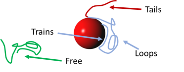 It says that if you place some particles, polymers and solvents within a notional lattice (a convenient fiction used widely in solution physics), and if you know the mutual interactions between components, you can work out where the polymer ends up, as "trains" in contact with the particle, "loops" which are the bulk of the polymer, "tails" which are the free ends sticking out, and "free" - the polymer unattached to the particle.
Most of us want polymers as stabilizers/dispersants for particles so we want plenty of polymer attached to the particle with plenty of tails sticking out (it's tails that provide steric stabilization), and with very little polymer "wasted" within the bulk of the solution.
This is easy to arrange in the app, but hard in reality because there are always tradeoffs. And that's why we have apps.
What's going on?
Start with Polymer A, just a single polymer. [In what follows I miss the letter A from the input names. When we come to B polymers, you just use the B equivalent.] You choose its length, N, in "lattice units" where 100 units is ~ 30nm extended length. As you will find, going to longer and longer polymers provides less and less impact and the app's pragmatic limit to the length is 1000 units. Now work out how it interacts with the solvent and how it and the solvent interact with the particles. We use the Flory-Huggins χ parameter for polymer/solvent, where 0 means they are very happy together and 0.5 is borderline. The relative liking of polymer and solvent for the particle is captured in χS named after Silberberg who decided that -1.5 means that the particle totally prefers the polymer and 0 means that it's neutral in its preference. You also have the volume fractions φ Particle and φ Polymer which describe the levels you add to the formulation.
As you slide the sliders (all non-relevant sliders are locked) you see what the polymer is doing. The X-axis is the number, Z, of lattice units away from the particle surface and the Y-axis shows the various volume fractions, φ at those positions. The φ All shows you the total amount of polymer, fading to φ Free which is the free polymer in the bulk solution (ideally this should be low). The φ T+L shows you the Trains (see the diagram above) and Loops, the bulk of the polymer which is generally coiled up. Then you see φ Tails which is the generally small fraction of polymer tails sticking out.
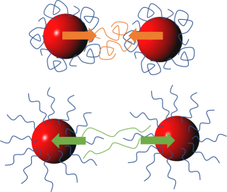 If you want stable particles then you want the polymer all on the particles and with (for interesting thermodynamic reasons) plenty of tails sticking out. Any polymer in the solution reduces stability ("bridging flocculation") because it tends to be coiled up and it's coils/loops that produce attraction (top diagram). This point about tails repelling and loops attracting is well-known to the specialist community but almost entirely unknown to the rest of us. We tend to show (lower diagram) bridging flocculation by extended polymers joining between tails, but this is totally wrong. Unfortunately, having a χ that encourages the tails to stick out might be incompatible with a χS which encourages the polymer to stay on the particle. Hence we use Di-Blocks and Combs.
Di-Blocks and Combs
Life becomes much easier if the A polymer loves the particle and hates the solvent and B is the other way round. You can now slide all the sliders, and the convention is to have χS for A to be, say, less than -1 and for the B equivalent to be near 0. The polymer A is near 0.5 and B near 0. The mutual like/dislike of the polymers is expressed as χA-B.
You can change the lengths of A and B to change the di-block behaviour and for combs you specify NCombs of length (usually modest) NB spaced equally along the main chain of length NA. If you go wild with NCombs and NB, be prepared for the calculation speed to become a problem. The speed does not depend on your laptop or phone - the calculations are all carried out on the server. This is the only one of my apps where that is the case as I prefer having everything client-side.
It's not immediately obvious, but combs are generally more effective than di-blocks. If you assume that the B polymer of the combs is essentially all tail and combine it with the thermodynamic fact that tails provide repulsion while loops encourage association, then things become clearer. For technical reasons we show All, A and B with no accounting for trains, loops and tails; and for combs we don't have the free value.
Two Polymers
It's not a good idea to mix polymers when you have particles stabilized by one of them. But formulators often have to add polymers that provide a specific functionality. Thanks to the power of SF theory we can explore what goes on. An ideal 2-polymer formulation is not easy to specify. For the A polymer to act as a good dispersant, it needs a χS near -1.5 and a modest χ. So what about the B? It needs a χS near 0 and a low χ. So the solvent has to rather like both A and B, yet A likes the particle and B doesn't. That's tricky.
The fact that tails repel and loops attract is a problem for 2-polymer systems. A will have lots of loops, because that's normal, and B will tend to have plenty of loops - and that can give bridging flocculation unles χA-B is large, meaning that the polymers don't want to interact much. This might cause subsequent problems in the dry formulation as the particles+polymer will not be well-integrated into the full system.
For those interested in depletion flocculation this app doesn't quite do the job. You need the full-powered version described below.
Grafted (Brush) Systems
My personal view is that formulators should always use a grafted or "brush" polymer. With no risk of polymer being removed, its solubility properties can be optimised for compatibility with the solvent and any other ingredients. For coating formulations, if the other end of the graft is a group that can react into the rest of the coating, things are even better.
Of course it's not so easy to make grafted systems, but formulators should at least discuss whether the problems of creating the graft are, in fact, less than problems caused by using conventional stabilizing systems.
In the app (which is technically a Planar Brush) you just specify NA, χA and the degree of grafting, φ Grafted. The output graph is very simple, just φ All. This current version may be less accurate at low graft levels - we are looking at tweaking the calculation for future upgrades.
χ Values
Where do the χ values comes from? My view is that the Hansen Solubility Parameter (HSP) approach is the most fertile. We all know that we can measure the HSP of polymers. It's less (but increasingly) well known that we can measure the HSP of particles. Knowing the HSP of the solvent then allows us to calculate HSP Distances between all the components. With a bit of imagination it's possible to calculate (or at least estimate) the χ, χA-B and χS values from these Distances. This is the approach adopted in the full-power version.
Other details
The SF calculations take place over a number of lattice layers. The app decides (on rational grounds) the relevant number of layers and NLayers is shown as an output. NLayers is usually rather more than you need for the polymer to reach equilibrium so you can choose the Z-Max of the plot - with the program displaying whichever is the minimum of NLayers and Z-Max. θ is the number of polymer segments which is effectively the number of layers occupied by polymer, the rest (NLayers-θ) being occupied by solvent. This value is required for the calculations (in "canonical system" mode) and is just a generally useful number to check from time to time. The Radius of Gyration, Rg is the number of lattice units typically occupied by a coiled polymer, provided also as a number in nm via a 0.3 conversion. It is a rough guide to the general thickness of the polymer on the particle.
Users will note that they don't specify a radius of the particle. It turns out that for most particles the curvature is sufficiently small that the assumption made in the app of a "planar" particle is good enough.
The calculations are only done at integer values of Z so the graphs would look rather unnatural if plotted directly. So the graphs have been artificially smoothed. Most of the time they look fine, but like all smoothing you might find some artefacts in some plots.
Full-Power SFBox-FE
The app represents a balance of power within the limits of an app format. For those who want more power, including the ability to handle larger polymers and to calculate particle-particle interactions, a full SFBox Front End has been added to the HSPiP software package. This makes sense because calculation of the various χ parameters can be done alongside measures of polymer and particle HSP values. The user can choose "live" calculations for smaller problems and swap to clicking a Calculate button for longer calculations, typically in the 2-6 second domain. The eBook that comes with HSPiP includes a longer explanation of SF theory.
Acknowledgements
The engine running on the server is SFBox from Prof Frans Leermakers of Wageningen U. His generosity for teaching me how to use SFBox and then allowing me to use it for the app is warmly acknowledged.
My introduction to SF theory was via Prof Terence Cosgrove of U Bristol and it's thanks to the historically strong Bristol-Wageningen links that SFBox-FE became possible. I'm grateful for that initial guidance and for helpful comments on the beta version of this app.
Getting the engine to run on my server was made possible by server genius Dr Jonathan Summers. Most people might have spent hours or days to set it up for me, but he managed it in (in his words) 5 minutes. Dr Summers has helped me many times over the years and I thank him yet again for his masterful assistance.
Lastly, I had no idea how to send the input data to SFBox and read the data output. Fortunately, Sean Cooper is a coding genius and sorted it out over a 1hr Zoom session. He even showed me how to de-bounce the inputs to reduce the server load and make the graph less jumpy. This is another occasion where I have to thank Sean for his amazing capabilities.
Of course, the responsibility for errors and glitches is entirely mine.
