Gravitational Sedimentation Calculator

The calculations here are based on the famous Mason & Weaver¹ paper from 1924. We have a column length l, a particle (or molecule) of radius r (and therefore volume V=4/3πr³) and density ρ (I use the absolute value of the difference, δ, so lighter particles seem to fall down...). For those with large polymers and biomaterials of known MWt, you can use the estimator² to find an appropriate equivalent radius. The solvent viscosity is η and the initial (relative) concentration is 1 down the length of the column. The temperature used for the kT value is fixed at 298 as its effect is small for typical cases.

A key trick in the Werts algorithm is to define a characteristic height, z₀ which we can calculate directly from our inputs:

`z_0=(3kT)/(4πrδg)` along with `z_(max)=l/z_0`

From these we get B which is the relative increase in concentration at the bottom at equilibrium, assuming a concentration of 1 at t=0:

`B=z_(max)/(z_0(1-exp((-z_(max))/z_0)))`

We also get a curve of concentration versus height,z, at infinite time:

`c(z)=B.exp((-z)/z_0)`

We need a diffusion coefficient D and a sedimentation coefficient s which, for convenience is defined with respect to D and z₀, and from which we can calculate the time to equilibrium:

`D=(kT)/(6πηr)` and `s=D/(z_0g)` and `t_(equil)=1.4z_(max)/(sg)`

The analytical solver takes those inputs, turns them into non-dimensional parameters (so the output plot is 0 to 100%) and then works out which of a number of analytical solutions applies to the specific set of non-dimensional constants.

Who cares?

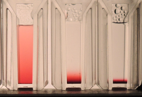Those who handle nanoparticles will benefit from exploring the app, for three reasons. First, it gives some idea of timescales. Second, and more importantly, because there is a big difference from this thermodynamic concentration gradient and "crashing out" of particles via, say, flocculation. It is important for the nanoparticle world to understand that gravity is not a way to distinguish "soluble" molecules from "dispersed" particles. A large DNA molecule behaves identically to a similar-sized nanoparticle. Thirdly because it's awesome to see a picture of the Boltzmann distribution. Yes, the curve at equilibrium is the Boltzmann distribution and this image of the red gold nanoparticles from the Werts' website (which also has lots of excellent Python scripts!) shows the equilibrium concentration for r=10, 20 and 30nm, l=15, ρ~20 with the water having a density of 1 and viscosity of 1.6. You can readily simulate them in the app.

Why is it the Boltzmann distribution? The equilibrium (which has nothing to do with Brownian motion) is between the chemical potential gradient of the gold particles and the gravitational potential. Gravity pulls the particles to a greater concentration, but that produces a counter-potential from concentration. The result is an exponential gradient governed by the Boltzmann constant k. As the Werts paper puts it, "The same result for the equilibrium gradient can be obtained using a statistical mechanical approach, i.e., calculating the Boltzmann distribution for dense suspended particles of buoyant mass m_b in a gravitationalfield (E_particle = m_bgz), illustrating that the digital image of the gold nanoparticle solution at equilibrium is a photograph of a Boltzmann distribution.". Or if we look again at the equation for the concentration versus depth this is:

`c(z)=B.exp((-z)/z_0) = B.exp((-z4πrδg)/(3kT)) = B.exp((-E)/(kT)) = "Boltzmann"`

The Werts experiments were done at 4°C (to minimize convection currents) but the app uses a fixed 25°C. Because kT is in °K, the difference of 277/298 in the exponential is not significant - and there's no room for a T slider!

But there's another amazing reason. Via a trick using osmotic membranes⁵, you can establish exactly the same gradient (i.e. the osmotic trick does not change the thermodynamics) in hours or days rather than months or years. So a 10cm column containing blue dextrin of MWt ~ 2million which would take years to settle normally, can produce a visible gradient in a day or so. This has been known for decades but has not been exploited recently - and deserves to be.