Solvent Blends

As discussed below, a blend of two solvents can often have better solubility properties (lower HSP Distance) than either of the individual solvents which might even be non-solvents for the target materials.

With this app you can try out these ideas. Choose a target polymer, then various pairs of solvents and vary their ratio till you get the best match (lowest HSP Distance or Ra). The evaporation graph will be discussed below:

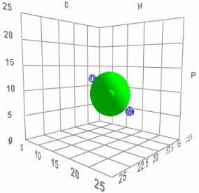When Charles Hansen first came up with his HSP scheme he saw that it made a surprising prediction. That two bad solvents (the blue dots in the image) on opposite sides of the HSP Sphere should produce an excellent solvent (green dot in the middle) when mixed 50:50. If his HSP ideas were wrong then mixing two bad solvents would create another bad solvent. When he did the test his ideas were confirmed - you really can make a good solvent from a mixture of bad ones.

This is probably the single most useful idea in the whole of HSP. It allows formulators amazing freedom to combine solvents that are attractive in terms of cost, safety, odour, volatility etc. but which are poor solvents for the specific system and create an excellent solvent blend.

For those who want a little more power, download HSP_Calculations.xlsx which allows optimization within Excel. For those who have sophisticated requirements such as automatic choice of the best three solvents from a list then the Solvent Optimizer within HSPiP is the perfect tool.

Evaporation tricks

By being smart with the relative volatilities of the solvents it's possible to make mixes that deliberately crash out the solutes when evaporation starts (the best solvent is more volatile) or crash out one solute component (the best solvent is more volatile) or, alternatively, to make a super-smooth coating by ensuring that the best solvent for the critical component is the least volatile so keeps it in solution up to the last moment.

Try this in the app. Choose two solvents of interest. Their RER (Relative Evaporation Rate) values are the last number shown in the square brackets. The evaporation graph shows the total amount of solvent (starting from 100%) and the % of each solvent during the evaporation process. It also plots the Ra value so you can see if solubility is getting better or worse. The evaporation time is arbitrary - just slide the slider till the evaporation process goes to completion. Why is it arbitrary? Because it depends on temperature, amount of solvent and, above all, air flow and turbulence. Such complexity is unnecessary to illustrate the key point which is that a rational solvent blend can add interesting extra capabilities to your formulation.

Polymer Effects

It seems obvious that if you start with, say, 20% solids then you have 20% less solvent so the solvent will disappear faster. Yet when you increase % solids you find that drying slows down! Why is this? I am grateful to Prof Wilhelm Schabel, Dr Philip Scharfer and Dipl-Eng Anna-Lena Riegel from the Karlsruhe Institute of Technology for introducing me to the Flory-Huggins entropy correction for the "activity" of the solvent (assuming that the solvent is "ideal" and that the solids are a polymer). With more and more polymer, there is an entropic driver to keep the solvent inside the polymer, so the effective vapour pressure decreases. Why not add an activity coefficient effect, especially a "repulsive" one when the solvent doesn't much like the polymer? Because, as they pointed out to me, the activity coefficient effect is strongly solvent-dependent involving at least a polynomial. That gets too complicated for the app.

The % of the least volatile solvent rises to 100% when there is no polymer present - it is 100% of the solvent blend. When polymer is present then the % is with respect to the total system which includes the solids. This explains why the plot changes alarmingly with a change from 0% to just a small % of solids.