
Noyes-Whitney Dissolution
Quick Start
To dissolve a tablet (typically for a pharmaceutical) you need the solute to leave the surface and diffuse across a zone into the bulk. The surface area and the concentration gradient both get smaller so the dissolution rate gets slower. The theory has been around since the 19th century but is good enough for the 21st.
Noyes-Whitney Dissolution
window.onload = function () {
    //restoreDefaultValues(); //Un-comment this if you want to start with defaults
     Main();
};

//Main() is hard wired as THE place to start calculating when inputs change
//It does no calculations itself, it merely sets them up, sends off variables, gets results and, if necessary, plots them.
function Main() {
    //Save settings every time you calculate, so they're always ready on a reload
    saveSettings();

    //Send all the inputs as a structured object
    //If you need to convert to, say, SI units, do it here!
    const inputs = {
        D: sliders.SlideD.value*1e-6, //cm2 units
        h: sliders.Slideh.value*1e-4, //μm to cm units
        rho: sliders.Sliderho.value, //keep in g.cc
        R: sliders.SlideR.value/10, //mm to cm
        H: sliders.SlideH.value/10, //mm to cm
        V: sliders.SlideV.value, //keep in cm3
        Csat: sliders.SlideCsat.value/1e3, //mg/ml to g/ml
        tmax: sliders.Slidetmax.value * 60, //min to s
        MWt: sliders.SlideMWt.value,
        eta: sliders.Slideeta.value, //Keep as cP for Wilke-Chang
   };


    //Send inputs off to CalcIt where the names are instantly available
    //Get all the resonses as an object, result
    const result = CalcIt(inputs);
    document.getElementById('Tmg').value = result.Tmg;
    document.getElementById('Dcalc').value = result.Dcalc;
    if (result.plots) {
        for (let i = 0; i < result.plots.length; i++) {
            plotIt(result.plots[i], result.canvas[i]);
        }
    }

    //You might have some other stuff to do here, but for most apps that's it for Main!
}

//Here's the app calculation
//The inputs are just the names provided - their order in the curly brackets is unimportant!
//By convention the input values are provided with the correct units within Main
function CalcIt({ D, h, rho, R, H, V, Csat, tmax, MWt, eta }) {
     let Sol = [], t=0
     const tstep=tmax/1000, PI=Math.PI, beta=H/R, Vs=PI*R*R*H, Cd=Vs*rho/V
     const K=D/h*Math.pow(Vs/rho,0.667)*2*PI*(1+2*beta)*Math.pow(1/(PI*beta),0.667)
     const Tmg=1000*Vs*rho
     //Diffusion coefficient via Modified Wilke-Chang
     const Dcalc=7.4e-8*Math.pow(2.26*18,0.5)*298/(eta*Math.pow(MWt,0.6))*1e6
     let C=0
     Sol.push({x:0,y:0})
    for (t = tstep; t<=tmax; t+=tstep) {
        //The max fixes tiny numerical glitches that can blow up
        C+=K*Math.pow(Math.max(Cd-C,0),0.667)*Math.max(Csat-C,0)*tstep
        Sol.push({x:t/60,y:C*1000})
        }
    //Now set up all the graphing data detail by detail.
    let plotData = [Sol]

    const prmap = {
        plotData: plotData, //An array of 1 or more datasets
        lineLabels: [], //An array of labels for each dataset
        colors: ["orange"], //An array of colors for each dataset
        borderWidth: [2,], //An array of line widths for each dataset
        hideLegend: true, //Set to true if you don't want to see any labels/legnds.
        xLabel: 't&min', //Label for the x axis, with an & to separate the units
        yLabel: 'C&mg/ml', //Label for the y axis, with an & to separate the units
        y2Label: null, //Label for the y2 axis, null if not needed
        yAxisL1R2: [], //Array to say which axis each dataset goes on. Blank=Left=1
        logX: false, //Is the x-axis in log form?
        xTicks: undefined, //We can define a tick function if we're being fancy
        logY: false, //Is the y-axis in log form?
        yTicks: undefined, //We can define a tick function if we're being fancy
        legendPosition: 'top', //Where we want the legend - top, bottom, left, right
        xMinMax: [0,], //Set min and max, e.g. [-10,100], leave one or both blank for auto
        yMinMax: [0, ], //Set min and max, e.g. [-10,100], leave one or both blank for auto
        y2MinMax: [,], //Set min and max, e.g. [-10,100], leave one or both blank for auto
        xSigFigs: 'F2', //These are the sig figs for the Tooltip readout. A wide choice!
        ySigFigs: 'F2', //F for Fixed, P for Precision, E for exponential
    };


    //Now we return everything - text boxes, plot and the name of the canvas, which is 'canvas' for a single plot
    return {
        Tmg: Tmg.toFixed(0)+ " : "+(Cd*1000).toPrecision(3),
        Dcalc: Dcalc.toFixed(1),
        plots: [prmap],
        canvas: ['canvas'],
    };
}
 Simple Diffusion
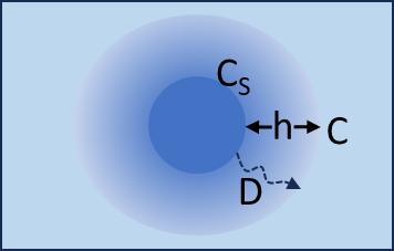
Molecules from the surface (area S) travel a distance h before they can be considered to be in the bulk solution. They have a diffusion coefficient D which you either know or can estimate from the MWt of the molecule and the viscosity of the solution.
If the saturated solution concentration is Cs and the bulk concentration (initially 0) is Cb then the rate of change of concentration, C, with time, t, is given by the Noyes-Whitney formula:
`(δC)/(δt)=(DS)/h(C_s-C_b)`
Because the surface area changes, you need to keep re-calculating S at each time step. A convenient formula for doing this was taken from Yanlei Kang, Jiahui Chen, Zhenyu Duan, and Zhong Li, Predicting Dissolution of Entecavir Using the Noyes-Whitney Equation, dx.doi.org/10.14227/DT300123P38. We assume a tablet of radius R and thickness H and of density ρ and that it is being dissolved in a volume V. From this we know the initial S, tablet mass and the final concentration that might be achieved if it all dissolves. These last two are shown as mg : mg/ml. We also need to know the saturated concentration which controls the rate and limits the process if it is lower than expected final concentration.
The diffusion coefficient can be estimated using the Wilke-Chang equation that depends on T (assumed to be 298K), MWt of the solvent (assumed to be 18), the MWt (strictly the Molar Volume) of the solute and η the viscosity of the solvent:
`D=(7.4e^(-8)(2.26MWt_(solv))^(0.5)T)/(ηMWt^0.6)`
The Diffusion Layer problem
Everything is known (or, in case of D, estimated) except h, the thickness of the diffusion layer. In reality it is obtained by fitting to a real dissolution curve. Values are typically a few 10s of μm. They depend, of course, on how well you are stirring. Typically it goes as `1/sqrt("rpm")` so a 40μm layer at 100 rpm would be 32μm at 150 rpm and 28μm at 200 rpm. In a quiescent gut, it might extend to 1000μm, hence the input slider is a log scale to cover this wide range.
If you apply Noyes-Whitney to powders then the relative velocity of the particles and, therefore, the mass transfer coefficient, will depend on, for example, relative densities. The consensus seems to be that particles that go with the flow have a -0.3 dependency on rpm, while more resistant ones might be closer to -0.8. Assuming -0.5 is, therefore, reasonable in the absence of precise information.
