
MSMPR Crystallizer
Quick Start
The Mixed-suspension, Mixed-Product-Removal (MSMPR) crystallizer is much used for large-scale inorganic crystallization and has a rather simple set of formulae linked to a rather complex set of processes. In this "reverse app" we input the answers and see the data, rather than in real life where we do the opposite. We compare a reference case (solid lines) with an alternative (dotted).
Credits
This is part of my series of apps on the complexities of crystallization. It is based on an example in the excellent Ch 6 by Åke Rasmuson in Handbook of Industrial Crystallization, 3rd Edition1.
MSMPR Crystallizer
//One universal basic required here to get things going once loaded
window.onload = function () {
    //restoreDefaultValues(); //Un-comment this if you want to start with defaults
    Main();
};
//Any global variables go here


//Main is hard wired as THE place to start calculating when input changes
//It does no calculations itself, it merely sets them up, sends off variables, gets results and, if necessary, plots them.
function Main() {
    saveSettings();

    //Send all the inputs as a structured object
    //If you need to convert to, say, SI units, do it here!
    const inputs = {
        g: sliders.Slideg.value,
        b: sliders.Slideb.value,
        j: sliders.Slidej.value,
        dS: sliders.SlidedS.value,
        dM: sliders.SlidedM.value,
        dQ: sliders.SlidedQ.value,
    }

    //Send inputs off to CalcIt where the names are instantly available
    //Get all the resonses as an object, result
    const result = CalcIt(inputs)

    //Set all the text box outputs
    document.getElementById('Comments').value = result.Comments
    //Do all relevant plots by calling plotIt - if there's no plot, nothing happens
    //plotIt is part of the app infrastructure in app.new.js
    if (result.plots) {
        for (let i = 0; i < result.plots.length; i++) {
            plotIt(result.plots[i], result.canvas[i]);
        }
    }

    //You might have some other stuff to do here, but for most apps that's it for CalcIt!
}

//Here's the app calculation
//The inputs are just the names provided - their order in the curly brackets is unimportant!
//By convention the input values are provided with the correct units within Main
function CalcIt({ g,b,j,dS,dM,dQ }) {

    let n1Curve = [], n2Curve = [],cn1Curve=[],cn2Curve=[],cv1Curve=[],cv2Curve=[]
    const n0=1e14,G0=1e-7,B0=n0*G0,t=1000
    const B1=B0*Math.pow(dM,j)*Math.pow(dS,g),n1=n0*B1/B0,G1=G0*Math.pow(dS,g),t1=t/dQ
    const Comments="n_0: "+n0.toExponential(2)+", B_0: "+B0.toExponential(2)+", G_0: "+G0.toExponential(2)+", Median_0: "+(1e6*3.67*G0*t).toPrecision(3)+"μm"+ " || n_1: "+n1.toExponential(2)+", B_1: "+B1.toExponential(2)+", G_1: "+G1.toExponential(2)+", Median_1: "+(1e6*3.67*G1*t1).toPrecision(3)+"μm"
    let n=0,cn1=0,cn2=0,cv1=0,cv2=0

    for (let L=0;L<=2000;L+=10){
        n=n0*Math.exp(-L*1e-6/(G0*t))
        if (L<=1000) n1Curve.push({x:L,y:Math.log(n)})
        cn1+=n
        if (L<=1000) cn1Curve.push({x:L,y:cn1})
        cv1+=n*Math.pow(L,3)
        if (L<=1000) cv1Curve.push({x:L,y:cv1})
        n=n1*Math.exp(-L*1e-6/(G1*t1))
        if (L<=1000) n2Curve.push({x:L,y:Math.log(n)})
        cn2+=n
        if (L<=1000) cn2Curve.push({x:L,y:cn2})
        cv2+=n*Math.pow(L,3)
        if (L<=1000) cv2Curve.push({x:L,y:cv2})
     }
     for (let i=0;i < cn1Curve.length;i++){
         cn1Curve[i].y/=cn1
         cn2Curve[i].y/=cn2
         cv1Curve[i].y/=cv1
         cv2Curve[i].y/=cv2
     }
    //Now set up all the graphing data detail by detail.

    const prmap = {
        plotData: [n1Curve,n2Curve,cn1Curve,cn2Curve,cv1Curve,cv2Curve],
        lineLabels: ["ln(n)_0","ln(n)_1","Cum.n_0","Cum.n_1","Cum.V_0","Cum.V_1"],
        dottedLine: [false, true, false, true, false,true],
        xLabel: "L&μm", //Label for the x axis, with an & to separate the units
        yLabel: "ln(n)&#/m.m³", //Label for the y axis, with an & to separate the units
        y2Label: "Cumulative", //Label for the y2 axis, null if not needed
        yAxisL1R2: [1,1,2,2,2,2], //Array to say which axis each dataset goes on. Blank=Left=1
        logX: false, //Is the x-axis in log form?
        xTicks: undefined, //We can define a tick function if we're being fancy
        logY: false, //Is the y-axis in log form?
        yTicks: undefined, //We can define a tick function if we're being fancy
        legendPosition: 'top', //Where we want the legend - top, bottom, left, right
        xMinMax: [0, 1000], //Set min and max, e.g. [-10,100], leave one or both blank for auto
        yMinMax: [,], //Set min and max, e.g. [-10,100], leave one or both blank for auto
        y2MinMax: [,], //Set min and max, e.g. [-10,100], leave one or both blank for auto
        xSigFigs: 'F3', //These are the sig figs for the Tooltip readout. A wide choice!
        ySigFigs: 'F3', //F for Fixed, P for Precision, E for exponential
    };

    //Now we return everything - text boxes, plot and the name of the canvas, which is 'canvas' for a single plot

    return {
        Comments: Comments,
        plots: [prmap],
        canvas: ['canvas'],
    };

}
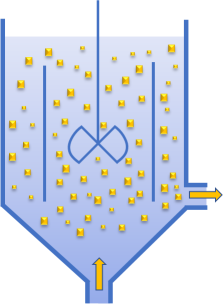 The Mixed-suspension, Mixed-Product-Removal (MSMPR) crystallizer is an amazing device. Saturated solution enters a chamber already full of crystals and an equal flow exits, containing whatever crystals exist at that end of the flow chamber. The image is of a DTB, Draft Tube Baffle configuration as one example. There is perfect mixing, zero breakage of crystals, no build-ups on walls or stirrers. Yes, it's an ideal, but especially for inorganic crystallizers, plenty of MSMPR systems work astonishingly well.
Our interest here is that unlike every other crystallizer, the equations are simple and the outcomes clear. Our reference system, with subscript 0, produces a population (per unit volume) n0=1E14 of seeds which grow at a rate G0 of 1e-7 m/s. This means that the nucleation rate B0=n0.G0 = 1e7/m³s. This is all happening with a saturation of S0, a mass of crystals M0 and a flow rate Q0.
The basic MSMPR equation tells us that after a time t (here assumed to be 1000s), for a crystal length L, the number of crystals with that size, nL is given by:
`n_L=n_0exp(-L/(Gt))`
So a plot of ln(nL) versus L is a nice straight line with slope -1/Gt and intercept n0. Of course in the real world the line isn't so perfect, but it is surprisingly common. The other core equations say that measures of "average" size are simple functions of Gt. In this app we get Lmedian which is just 3.67Gt, in this case 367μm.
Because this is a log plot we see that the system is dominated by small crystals. But as is often the case with particle sizes, this is something of an illusion. From the cumulative number distribution 70% of the crystals are (move your mouse over the line to see this) less than 110μm. But we are usually more interested in the crystal as a whole, so it's the volume or mass distribution that interests us. When that's plotted we see that there are an equal number below ~360μm as above, i.e. our calculated Lmedian value.
Changes to the parameters
The specific reference values will be of no interest. Making them a user option would just complicate the interface. The point of the app is to show the general MSMPR equation then to look at the effects of process variables - saturation, mass of crystals ("magma") in the reactor and the flow rate. You set up a second set of conditions, with subscript 1, by changing ΔS, ΔM and ΔQ, relative changes (by a factor of 5 more or less) in those parameters. You then see the second straight MSMPR line along with the number and volume cumulative distributions. The change with ΔQ is straightforward, it's just changing t, the time spent in the reactor.
The other reason for the app is that different crystallizations show different power law dependencies for ΔS and ΔM on the the growth rate G and the nucleation rate B.
`G_1=G_0(ΔS)^g`
`B_1=B_0(ΔS)^b(ΔM)^j`
In the book chapter example, g=1.58, b=2.09 and j=1. Any process with a power law dependence much above 1 is likely to be challenging. If you set these three parameters to 1, then changes to saturation or mass lead to orderly changes in the crystals. But once one or more is above 2 then small changes get amplified - and that's a key problem with real-world crystallization. Here we are merely modelling an ideal single stage. In practice the crystallizers will be multi-stage, and their mixing (and therefore degree of saturation) isn't perfect, removal of crystals isn't size-independent, and models don't (can't) cope with issues such as size-dependent or crystal-dependent growth rates.
Real world data
If you were doing this for real, where would you get the reference data and how would you work out the various power laws? The answer, as with everything in crystallization is that it isn't easy. A lab-scale MSMPR reactor is surprisingly hard to construct so you have to try to get representitive values from simplified experiments. Then you have to do your best to fit your process data to get as good an idea as possible about what's happening. It's not perfect, but it's better than twiddling buttons with the hope that things will get better.
Åke C. Rasmuson, Ch 6 Crystallization Process Analysis by Population Balance Modeling in Allan S. Myerson, Deniz Erdemir, Alfred Y. Lee, Handbook of Industrial Crystallization, 3rd Edition, Cambridge U Press, 2019
