Isotherms via Statistical Thermodynamics

Quick Start

Isotherms are often described and interpreted by models such as Langmuir, BET or GAB that themselves contain assumptions that are often invalid. We can model many typical isotherms via a single, assumption-free theory using statistical thermodynamics. There is a simpler version for those interested specifically in Food Isotherms.

Credits

The app is based on the core paper by Shimizu and Matubayasi1 and subsequent papers with co-authors Dalby, Harton and Abbott2-4.

Isotherms-ST

A × 1000
B × 1000
C × 1000
D x 1000
amax
Fit Quality
Model
Convert
⟨n2⟩ Units
Standard values
Sorbate; MWt; Ų
T °C
//One universal basic required here to get things going once loaded
window.onload = function () {
    //restoreDefaultValues(); //Un-comment this if you want to start with defaults
    document.getElementById('Load').addEventListener('click', clearOldName, false);
    document.getElementById('Load').addEventListener('change', handleFileSelect, false);
    document.getElementById('Reverse').addEventListener("click", DoModel)
    // document.getElementById('Parameters').addEventListener('change', DoModel, false);
    Main();
};
//Any global variables go here
let amUpdating = false, lastFit = "", newFit = false, lastQ = 0, lastUnits = "", lastProbe = "", lastT = 0, divBy = 1, ModelLabel = "Model Parameters", G22conv = 1
let fitData = [], naFitData = [], scaleData = [], Loading = false, oldParams = ""

//Main is hard wired as THE place to start calculating when input changes
//It does no calculations itself, it merely sets them up, sends off variables, gets results and, if necessary, plots them.
function Main() {
    if (amUpdating) return
    saveSettings();
    if (Loading) return
    //Send all the inputs as a structured object
    //If you need to convert to, say, SI units, do it here!
    const inputs = {
        A: sliders.SlideA.value,
        B: sliders.SlideB.value,
        C: sliders.SlideC.value,
        D: sliders.SlideD.value,
        amax: sliders.Slideamax.value,
        Q: sliders.SlideQ.value,
        Probe: document.getElementById('Probe').value,
        T: sliders.SlideT.value,
        Units: document.getElementById('Units').value,
        Model: document.getElementById('Model').value,
    }

    //Send inputs off to CalcIt where the names are instantly available
    //Get all the resonses as an object, result
    if (!amUpdating && document.getElementById('Model').value.includes("File")) console.time("Calc")
    const result = CalcIt(inputs)
    if (!amUpdating && document.getElementById('Model').value.includes("File")) console.timeEnd("Calc")

    //Set all the text box outputs
    // document.getElementById('Langmuir').value = result.Lang
    document.getElementById('Parameters').value = result.Parameters
    document.getElementById('Values').value = result.Values
    document.getElementById('ModelLabel').innerHTML = result.ModelLabel
    oldParams = document.getElementById('Parameters').value
    //Do all relevant plots by calling plotIt - if there's no plot, nothing happens
    //plotIt is part of the app infrastructure in app.new.js
    if (result.plots) {
        for (let i = 0; i < result.plots.length; i++) {
            plotIt(result.plots[i], result.canvas[i]);
        }
    }

    //You might have some other stuff to do here, but for most apps that's it for CalcIt!
}
function DoModel() {
    const theModel = document.getElementById('Model').value
    const params = document.getElementById('Parameters').value
    const vals = params.split(/:| |,/)
    let A, B, C, tmp = []
    if (theModel == "GAB") {
        tmp = gettmp(vals)
        if (tmp.length == 3) {
            const nm = tmp[0]
            const CB = tmp[1]
            const K = tmp[2]
            A = 1 / (CB * K * nm); B = (2 - CB) / (CB * nm); C = (2 * K * (CB - 1)) / (CB * nm)
            amUpdating = true
            sliders.SlideA.value = A
            sliders.SlideB.inputValue = B
            sliders.SlideC.inputValue = C
            amUpdating = false
        }
    }
    if (theModel == "BET") {
        tmp = gettmp(vals)
        if (tmp.length == 3) {
            const nm = tmp[0]
            const CB = tmp[1]
            const K = tmp[2]
            A = 1 / (CB * K * nm); B = (2 - CB) / (CB * nm); C = (2 * K * (CB - 1)) / (CB * nm)
            amUpdating = true
            sliders.SlideA.value = A
            sliders.SlideB.inputValue = B
            sliders.SlideC.inputValue = C
            amUpdating = false
        }
    }
    if (theModel == "Hailwood-Horrobin") {
        tmp = gettmp(vals)
        if (tmp.length == 3) {
            A = tmp[0]
            B = tmp[1]
            C = tmp[2]
            amUpdating = true
            sliders.SlideA.value = A
            sliders.SlideB.value = -B
            sliders.SlideC.value = 2 * C
            amUpdating = false
        }
    }
    if (theModel == "Langmuir") {
        tmp = gettmp(vals)
        if (tmp.length == 2) {
            const nm = tmp[0], K1 = tmp[1]
            A = 1 / (nm * K1)
            B = 1 / nm
            sliders.SlideA.value = A
            sliders.SlideB.value = -B
        }
    }
    Main()
}
function gettmp(vals) {
    let i = 0, tmp = []
    for (i = 0; i < vals.length; i++) {
        if (vals[i] != "" && !isNaN(vals[i])) tmp.push(parseFloat(vals[i]))
    }
return tmp
}
//Here's the app calculation
//The inputs are just the names provided - their order in the curly brackets is unimportant!
//By convention the input values are provided with the correct units within Main
function CalcIt({ A, B, C, Q, amax, Model, Probe, Units, T }) {
    if (oldParams != "" && document.getElementById('Parameters').value != oldParams) {
        oldParams = document.getElementById('Parameters').value
        return { Parameters: document.getElementById('Parameters').value }
    }
    let FQ = 2000 + 2000 * Q * Q
    if (document.getElementById('SlideQ').style.visibility == "hidden") FQ = 10000
    if (Model == "File A-B-C-D Fit") FQ = 2000 + 2000 * Math.pow(Q, 1.5) //ABCD can be very slow
    const ProbeData = Probe.split(";")
    const MWt = parseFloat(ProbeData[1])
    const Area = parseFloat(ProbeData[2])
    const AA = parseFloat(ProbeData[3])
    const AB = parseFloat(ProbeData[4])
    const AC = parseFloat(ProbeData[5])
 
    if (amUpdating) return { Parameters: "-" }
    document.getElementById('Load').disabled = !Model.includes("File")
    //if (Model == lastFit) return { Parameters: "-" }
    if (Model == "-None-" || Model == "Peleg" || Model == "Freundlich" || Model == "Fractal-FHH" || Model == "Oswin" || Model == "Dubinin-Radushkevich" || Model == "Halsey" || Model == "Henderson" || Model == "Bradley"|| Model == "File A-B-C-D Fit") {
        document.getElementById('SlideC').style.visibility = "visible"
        document.getElementById('SlideD').style.visibility = "visible"
        document.getElementById('Parameters').readOnly = true

    } else {
        amUpdating = true
        if (Model.includes("File")) {
            document.getElementById('Parameters').readOnly = true

        } else {
            document.getElementById('Parameters').readOnly = false

        }
        if (Model == "Langmuir" || Model == "File A-B Fit") {
            sliders.SlideC.inputValue = 0
            C = 0
            document.getElementById('SlideC').style.visibility = "hidden"
        }
        else {
            document.getElementById('SlideC').style.visibility = "visible"
        }
        sliders.SlideD.inputValue = 0
        D = 0
        document.getElementById('SlideD').style.visibility = "hidden"
        amUpdating = false
    }
    if (Model.includes("File")) {
        document.getElementById('SlideQ').style.visibility = "visible"
    } else {
        document.getElementById('SlideQ').style.visibility = "hidden"

        Loading = false
    }
    // document.getElementById('Reverse').disabled==document.getElementById('Parameters').readOnly
    const RT = 8.314 * (T + 273.15)
    let ICurve = [], GCurve = [], NCurve = [], anCurve = [], PCurve = [], naCurve = [], G22 = 0, n = 0, E = 0, F = 0, G = 0, H = 0
    let Parameters = "-", Values = "-"
    const a2inc = (Model == "Fractal-FHH" || Model == "Freundlich") ? 0.005 : 0.01
    if (!Model.includes("File")) {
        fitData = []; naFitData = []
        clearOldName()
        Loading = false
    }
    ModelLabel = "Model Parameters"
    document.getElementById('Clabel').innerHTML = "C × 1000"
    //Handle the Files first
    let xmax = amax - 0.05
    let conv = 1
    if (!Units.includes("mol")) conv *= MWt
    if (Units.includes("/g")) conv /= 1000
    if (Units.includes("/100g")) conv /= 10

    if (Model.includes("File") && fitData.length > 3) {
        document.getElementById('Slideamax').style.visibility = "hidden"
        let x = [], y = []
        naFitData = []
        for (let i = 0; i < fitData.length; i++) {
            x[i] = fitData[i].x
            y[i] = fitData[i].y
            if (x[i] > 0.025) naFitData.push({ x: fitData[i].x, y: fitData[i].y * divBy / fitData[i].x })
        }
        xmax = parseFloat(x[fitData.length - 1])
        if (amax < xmax) amax = Math.min(1, xmax + 0.05) // Users can choose to have a higher value but not a lower one
        if (newFit || Q != lastQ || Probe != lastProbe || Units != lastUnits || lastFit != Model) {
            lastFit = Model; lastQ = Q; lastUnits = Units; lastProbe = Probe
            amUpdating = true
            if (Model.includes("A-B Fit")) {
                PFunc = function (x, P) {
                    return x.map(function (xi) {
                        return xi / (P[0] - P[1] * xi)
                    })
                }
                var Parms = fminsearch(PFunc, [1, -1], x, y, {
                    maxIter: FQ
                })
                A = Parms[0]; B = Parms[1]; C = 0; D = 0
                sliders.SlideA.value = A
                sliders.SlideB.value = B
            }
            if (Model.includes("A-B-C Fit")) {
                PFunc = function (x, P) {
                    return x.map(function (xi) {
                        return xi / (P[0] - P[1] * xi - P[2] / 2 * xi * xi)
                    })
                }
                var Parms = fminsearch(PFunc, [1, -5, 5], x, y, {
                    maxIter: FQ
                })

                A = Parms[0]; B = Parms[1]; C = Parms[2]; D = 0
                sliders.SlideA.value = A
                sliders.SlideB.value = B
                sliders.SlideC.value = C
            }
            if (Model.includes("A-B-C-D Fit")) {
                PFunc = function (x, P) {
                    return x.map(function (xi) {
                        return xi / (P[0] - P[1] * xi - P[2] / 2 * xi * xi - P[3] / 3 * xi * xi * xi)
                    })
                }
                var Parms = fminsearch(PFunc, [1, -1, 1, 1], x, y, {
                    maxIter: FQ
                })
                A = Parms[0]; B = Parms[1]; C = Parms[2]; D = Parms[3]
                sliders.SlideA.value = A
                sliders.SlideB.value = B
                sliders.SlideC.value = C
                sliders.SlideD.value = D
            }
            if (Model.includes("Type IV")) {
                //Although Type IV data can be fitted by the native formula
                //the fitting can be re-cast using 3 parameters from the curve itself
                //This is both faster and likely to have fewer fitting artefacts.
                PFunc = function (x, P) {
                    return x.map(function (xi) {
                        // return P[0] * (P[1] * xi) / (1 + P[1] * xi) + P[2] * (P[3] * P[4] * Math.pow(xi, P[3])) / (1 + P[4] * Math.pow(xi, P[3]))
                        return P[0] * (P[1] * xi) / (1 + P[1] * xi) + P[2] * (P[3] * Math.exp(P[3] * (P[4] + Math.log(xi)))) / (1 + Math.exp(P[3] * (P[4] + Math.log(xi))))
                    })
                }
                let dmax = 0, a2mid = 0
                for (i = 1; i < y.length; i++) {
                    tmp = (y[i] - y[i - 1]) / (x[i] - x[i - 1])
                    if (isFinite(tmp) && tmp > dmax) { dmax = tmp; a2mid = x[i] }
                }
                const h = Math.max(...y)
                let xval = 1, N = 1, m = 40
                //The values from the curve - assuming they make sense
                if (a2mid > 0.1 && a2mid < 0.9 && dmax > 0) {
                    xval = -Math.log(a2mid)
                    N = h * h / (4 * dmax * a2mid)
                    m = h / N
                }
                // var Parms = fminsearch(PFunc, [0.5, 1, 1, 5, 1000], x, y, {
                //     maxIter: FQ, noNeg:true
                //  })
                // A = Parms[0]; B = Parms[1]; C = Parms[2]; D = Parms[3]; E = Parms[4]
                var Parms = fminsearch(PFunc, [0.5, 1, N, m, xval], x, y, {
                    maxIter: FQ, noNeg: true
                })
                //Am comes from the combination of xval and m
                A = Parms[0]; B = Parms[1]; C = Parms[2]; D = Parms[3]; E = Math.exp(Parms[3] * Parms[4])
                let conv = 1
                if (!Units.includes("mol")) conv *= MWt
                if (Units.includes("/g")) conv /= 1000
                if (Units.includes("/100g")) conv /= 10
                Parameters = "Na : " + (A * divBy / conv).toPrecision(3) + " mol/kg, A1 : " + B.toPrecision(3) + " Nb : " + (C * divBy / conv).toPrecision(3) + " mol/kg, m : " + D.toPrecision(4) + ", Am : " + E.toPrecision(4)
                let cText = (A * divBy / conv).toPrecision(3) + '\t' + B.toPrecision(3) + '\t' + (C * divBy / conv).toPrecision(4) + '\t' + D.toPrecision(4) + '\t' + E.toPrecision(4)
                copyTextToClipboard(cText)
            }
            if (Model.endsWith("Type V")) {
                PFunc = function (x, P) {
                    return x.map(function (xi) {
                        return P[0] * (P[1] * xi + P[3] * P[2] * Math.pow(xi, P[3])) / (1 + P[1] * xi + P[2] * Math.pow(xi, P[3]))
                    })
                }
                const ymax = Math.max(...y)
                var Parms = fminsearch(PFunc, [ymax / 10, 1, 100, 10], x, y, {
                    maxIter: FQ, noNeg: true
                })

                A = Parms[0]; B = Parms[1]; C = Parms[2]; D = Parms[3]; E = 0
                let conv = 1
                if (!Units.includes("mol")) conv *= MWt
                if (Units.includes("/g")) conv /= 1000
                if (Units.includes("/100g")) conv /= 10
                Parameters = "N : " + (A * divBy / conv).toPrecision(3) + " mol/kg, m : " + D.toPrecision(3) + ", A1 : " + B.toPrecision(3) + ", Am : " + C.toPrecision(4)
                let cText = (A * divBy / conv).toPrecision(3) + '\t' + D.toPrecision(3) + '\t' + B.toPrecision(3) + '\t' + C.toPrecision(4)
                copyTextToClipboard(cText)
            }
            if (Model.endsWith("Type VI")) {
                PFunc = function (x, P) {
                    return x.map(function (xi) {
                        return P[0] * (P[1] * xi) / (1 + P[1] * xi) + P[2] * (P[3] * P[4] * Math.pow(xi, P[3])) / (1 + P[4] * Math.pow(xi, P[3])) + P[5] * (P[6] * P[7] * Math.pow(xi, P[6])) / (1 + P[7] * Math.pow(xi, P[6]))
                    })
                }
                const ymax = Math.max(...y)
                var Parms = fminsearch(PFunc, [0.5, 1, 0.005, 5, 1000, 0.0005, 30, 10000], x, y, {
                    maxIter: FQ, noNeg: true
                })
                A = Parms[0]; B = Parms[1]; C = Parms[2]; D = Parms[3]; E = Parms[4]; F = Parms[5]; G = Parms[6]; H = Parms[7]
                let conv = 1
                if (!Units.includes("mol")) conv *= MWt
                if (Units.includes("/g")) conv /= 1000
                if (Units.includes("/100g")) conv /= 10
                Parameters = "Na : " + (A * divBy / conv).toPrecision(3) + " mol/kg, A1 : " + B.toPrecision(3) + " Nb : " + (C * divBy / conv).toPrecision(3) + " mol/kg, m : " + D.toPrecision(3) + ", Am : " + E.toPrecision(3) + " Nc : " + (F * divBy / conv).toPrecision(3) + " mol/kg, n : " + G.toPrecision(3) + ", An : " + H.toPrecision(3)
                let cText = (A * divBy / conv).toPrecision(3) + '\t' + B.toPrecision(3) + '\t' + (C * divBy / conv).toPrecision(4) + '\t' + D.toPrecision(3) + '\t' + E.toPrecision(3) + '\t' + (F * divBy / conv).toPrecision(4) + '\t' + G.toPrecision(3) + '\t' + H.toPrecision(3)
                copyTextToClipboard(cText)
            }
            amUpdating = false
            let cText = (conv * A / divBy).toPrecision(4) + '\t' + (conv * B / divBy).toPrecision(4)
            if (Math.abs(C) > 0.001) cText += '\t' + (conv * C / divBy).toPrecision(4)
            if (Math.abs(D) > 0.001) cText += '\t' + (conv * D / divBy).toPrecision(4)
            if (Math.abs(E) > 0.001) cText += '\t' + (conv * E / divBy).toPrecision(4)
            if (!Model.includes("Type")) copyTextToClipboard(cText)
            let sText = "A: " + (conv * A / divBy).toPrecision(4) + ' B: ' + (conv * B / divBy).toPrecision(4)
            if (Math.abs(C) > 0.001) sText += ' C: ' + (conv * C / divBy).toPrecision(4)
            if (Math.abs(D) > 0.001) sText += ' D: ' + (conv * D / divBy).toPrecision(4)
            if (Math.abs(E) > 0.001) sText += ' E: ' + (conv * E / divBy).toPrecision(4)
            if (Model.includes("File") && fitData.length > 3) sText += ' -B/C:' + (-B / C).toPrecision(3)
            if (!Model.includes("Type")) { Parameters = sText }
            // conv = 1
            ModelLabel = "Model Parameters"
            if (Model.includes("File") && !Model.includes("Type") && fitData.length > 3) {
                ModelLabel = "Model Parameters kg/mol"
                const VPRT = isNaN(AA) ? "-" : Math.pow(10, AA - AB / (AC + T)) / 760 * 100000 / (8.312 * (T + 273.15))
                const Gs2 = divBy / (conv * VPRT * A)
                const G22 = conv * B / divBy
                const VSA = -Area * 1e-20 * 6.02e23 / G22 / 1000 //Decided to do it /g instead of /kg
                if (VPRT == "-") {
                    Values = "STSA = " + VSA.toPrecision(3) + " m²/g"
                } else {
                    Values = "Gs2° = " + Gs2.toPrecision(4) + " m³/kg, G22°/v° = " + G22.toPrecision(4) + " kg/mol, STSSA = " + VSA.toPrecision(3) + " m²/g, c2_sat = " + VPRT.toPrecision(3) + " mol/m³"
                }
            }
            G22conv = conv
            newFit = false
        }
    } else {
         if ( Model == "Hailwood-Horrobin" || Model == "Langmuir" || Model == "GAB" || Model == "BET") {
            ModelLabel = "Model Parameters kg/mol"
            const VPRT = isNaN(AA) ? "-" : Math.pow(10, AA - AB / (AC + T)) / 760 * 100000 / (8.312 * (T + 273.15))
            const Gs2 = divBy / (conv * VPRT * A)
            const G22 = conv * B / divBy
            const VSA = -Area * 1e-20 * 6.02e23 / G22 / 1000 //Decided to do it /g instead of /kg
            if (VPRT == "-") {
                Values = "STSA = " + VSA.toPrecision(3) + " m²/g"
            } else {
                Values = "Gs2° = " + Gs2.toPrecision(4) + " m³/kg, G22°/v° = " + G22.toPrecision(4) + " kg/mol, STSSA = " + VSA.toPrecision(3) + " m²/g, c2_sat = " + VPRT.toPrecision(3) + " mol/m³"
            }
        }
        document.getElementById('Slideamax').style.visibility = "visible"
        lastFit = ""; divBy = 1
    }

    for (let a2 = a2inc; a2 <= Math.min(amax, xmax + 0.05); a2 += a2inc) {
        if (!Model.includes("Type")) {
            n = a2 / (A - E * Math.pow(a2, 4) / 4 - D * Math.pow(a2, 3) / 3 - C * Math.pow(a2, 2) / 2 - B * a2)
            G22 = E * a2 * a2 * a2 + D * a2 * a2 + C * a2 + B

        } else {
            if (Model.endsWith("Type IV")) {
                n = A * B * a2 / (1 + B * a2) + C * (D * E * Math.pow(a2, D)) / ((1 + E * Math.pow(a2, D)))
                G22 = C * D * D * E * Math.pow(a2, D - 1) / (E * Math.pow(a2, D) + 1) - C * D * D * E * E * Math.pow(a2, 2 * D - 1) / Math.pow(E * Math.pow(a2, D) + 1, 2) + A * B / (B * a2 + 1) - A * B * B * a2 / Math.pow(B * a2 + 1, 2)
            }
            if (Model.endsWith("Type V")) {
                n = A * (B * a2 + 2 * E * Math.pow(a2, 2) + D * C * Math.pow(a2, D)) / (1 + B * a2 + E * Math.pow(a2, 2) + C * Math.pow(a2, D))
                G22 = -1 / A + D * (D - 1) / A * C * (1 + B * a2 + C * Math.pow(a2, D)) * Math.pow(a2, D - 2) / Math.pow(B + D * C * Math.pow(a2, D - 1), 2)
            }
            if (Model.endsWith("Type VI")) {
                n = A * B * a2 / (1 + B * a2) + C * (D * E * Math.pow(a2, D)) / ((1 + E * Math.pow(a2, D))) + F * (G * H * Math.pow(a2, G)) / ((1 + H * Math.pow(a2, G)))
                G22 = F * G * G * H * Math.pow(a2, G - 1) / (H * Math.pow(a2, G) + 1) - F * G * G * H * H * Math.pow(a2, 2 * G - 1) / Math.pow(H * Math.pow(a2, G) + 1, 2) + C * D * D * E * Math.pow(a2, D - 1) / (E * Math.pow(a2, D) + 1) - C * D * D * E * E * Math.pow(a2, 2 * D - 1) / Math.pow(E * Math.pow(a2, D) + 1, 2) + A * B / (B * a2 + 1) - A * B * B * a2 / Math.pow(B * a2 + 1, 2)
            }
        }
        if (n > 1 || n < -0.02) break
        ICurve.push({ x: a2, y: Math.max(0, n * divBy) })
        GCurve.push({ x: a2, y: G22conv * G22 / divBy })
        NCurve.push({ x: a2, y: G22conv * G22 * n * divBy })
        if (a2 > 0.025) naCurve.push({ x: a2, y: Math.max(0, n * divBy) / a2 })
        if (n * divBy > 0.025) anCurve.push({ x: a2, y: a2 / (n * divBy) })
    }
    //Rounding error issues for the plot
    n = amax / (A - E * Math.pow(amax, 4) / 4 - D * Math.pow(amax, 3) / 3 - C * Math.pow(amax, 2) / 2 - B * amax)
    if (!Model.includes("Type")) {
        n = amax / (A - E * Math.pow(amax, 4) / 4 - D * Math.pow(amax, 3) / 3 - C * Math.pow(amax, 2) / 2 - B * amax)
    } else {
        if (Model.endsWith("Type IV")) {
            n = A * B * amax / (1 + B * amax) + C * (D * E * Math.pow(amax, D)) / ((1 + E * Math.pow(amax, D)))
        }
        if (Model.endsWith("Type V")) {
            n = A * (B * amax + +  2 * E * Math.pow(amax, 2) + D * C * Math.pow(amax, D)) / (1 + B * amax + E * Math.pow(amax, 2) + C * Math.pow(amax, D))
        }
        if (Model.endsWith("Type VI")) {
            n = A * B * amax / (1 + B * amax) + C * (D * E * Math.pow(amax, D)) / ((1 + E * Math.pow(amax, D))) + F * (G * H * Math.pow(amax, G)) / ((1 + H * Math.pow(amax, G)))
        }
    }

    if (xmax + 0.05 >= amax && n <= 1 && n > 0) ICurve.push({ x: amax, y: n * divBy })

    if (Model == "Hailwood-Horrobin") {
        Parameters = "A: " + (A / divBy).toPrecision(3) + ", B: " + -(B / divBy).toPrecision(3) + ", C: " + (C / divBy / 2).toPrecision(3)
    }

    if (Model == "ABC") {
        Parameters = "A: " + (A / divBy).toPrecision(3) + ", B: " + (B / divBy).toPrecision(3) + ", C: " + (C / divBy).toPrecision(3)
    }

    if (Model == "Langmuir") {
        const nm = -1 / B, Kl = 1 / (nm * A)
        Parameters = "K1: " + nm.toPrecision(3) + ", K2: " + Kl.toPrecision(3)
    }
    if (Model == "GAB") {
        //Solve a quadratic to get the values
        const ab = C * A, bb = -4 * C * A - 2 * B * B, cb = 4 * C * A + 2 * B * B
        const GC = (-bb + Math.sqrt(bb * bb - 4 * ab * cb)) / (2 * ab)
        const GM = (2 - GC) / (B * GC)
        const GK = B / (A * (2 - GC))
        Parameters = "nm: " + GM.toPrecision(3) + " CB: " + GC.toPrecision(3) + " K: " + GK.toPrecision(3)
    }
    if (Model == "BET") {
        document.getElementById('SlideC').style.visibility = "hidden"
        document.getElementById('Clabel').innerHTML = "C = 2(A-B)"
        const BC = 2 * A - 2 * B
        amUpdating = true
        sliders.SlideC.inputValue = BC
        amUpdating = false
        //Solve a quadratic to get the values
        const ab = BC * A, bb = -4 * BC * A - 2 * B * B, cb = 4 * BC * A + 2 * B * B
        const GC = (-bb + Math.sqrt(bb * bb - 4 * ab * cb)) / (2 * ab)
        const GM = (2 - GC) / (B * GC)
        const GK = B / (A * (2 - GC))
        Parameters = "nm:" + GM.toPrecision(3) + " CB: " + GC.toPrecision(3) + " K: " + GK.toPrecision(3)
    }
    if (Model == "Peleg") {
        PFunc = function (x, P) {
            return x.map(function (xi) {
                return P[0] * Math.pow(xi, P[1]) + P[2] * Math.pow(xi, P[3])
            })
        }
        let x = [], y = []
        for (let i = 0; i < ICurve.length; i++) {
            x[i] = ICurve[i].x
            y[i] = ICurve[i].y
        }
        var Parms = fminsearch(PFunc, [1, 0.8, -1, 0.8], x, y, {
            maxIter: FQ/2
        })
        Parameters = "K1: " + Parms[0].toPrecision(3) + ", N1: " + Parms[1].toPrecision(3) + ", K2: " + Parms[2].toPrecision(3) + ", N2: " + Parms[3].toPrecision(3)
        for (let i = 0; i < ICurve.length; i++) {
            PCurve.push({ x: x[i], y: PFunc([x[i]], Parms)[0] * divBy })
        }
    }
    if (Model == "Fractal-FHH") {
        PFunc = function (x, P) {
            return x.map(function (xi) {
                return P[0] * Math.pow(-RT * Math.log(xi), P[1] - 3)
            })
        }
        let x = [], y = []
        for (let i = 0; i < ICurve.length; i++) {
            if (ICurve[i].x > 0) { //Don't want logs of near-zero
                x.push(ICurve[i].x)
                y.push(ICurve[i].y)
            }

        }
        var Parms = fminsearch(PFunc, [10, 2.5], x, y, {
            maxIter: FQ
        })
        Parameters = "K1: " + Parms[0].toPrecision(3) + ", D: " + Parms[1].toPrecision(3)
        for (let i = 0; i < x.length; i++) {
            PCurve.push({ x: x[i], y: PFunc([x[i]], Parms)[0] * divBy })
        }
    }
    if (Model == "Oswin") {
        PFunc = function (x, P) {
            return x.map(function (xi) {
                return P[0] * Math.pow(xi / (1 - xi), P[1])
            })
        }
        let x = [], y = []
        for (let i = 0; i < ICurve.length; i++) {
            if (ICurve[i].x <= 0.95) {
                x.push(ICurve[i].x)
                y.push(ICurve[i].y)
            }
        }
        var Parms = fminsearch(PFunc, [1, 1], x, y, {
            maxIter: FQ
        })
        Parameters = "K1: " + Parms[0].toPrecision(3) + ", N: " + Parms[1].toPrecision(3)
        for (let i = 0; i < x.length; i++) {
            PCurve.push({ x: x[i], y: PFunc([x[i]], Parms)[0] * divBy })
        }
    }
    if (Model == "Smith") {
        PFunc = function (x, P) {
            return x.map(function (xi) {
                return P[0] - P[1] * Math.log((1 - xi))
            })
        }
        let x = [], y = []
        for (let i = 0; i < ICurve.length; i++) {
            if (ICurve[i].x <= 0.95) {
                x.push(ICurve[i].x)
                y.push(ICurve[i].y)
            }
        }
        var Parms = fminsearch(PFunc, [1, 1], x, y, {
            maxIter: FQ
        })
        Parameters = "K1: " + Parms[0].toPrecision(3) + ", K2: " + Parms[1].toPrecision(3)
        for (let i = 0; i < x.length; i++) {
            PCurve.push({ x: x[i], y: PFunc([x[i]], Parms)[0] * divBy })
        }
    }
    if (Model == "Freundlich") {
        PFunc = function (x, P) {
            return x.map(function (xi) {
                return P[0] * Math.pow(xi, 1 / P[1])
            })
        }
        let x = [], y = []
        for (let i = 0; i < ICurve.length; i++) {
            if (ICurve[i].x <= 0.95) {
                x.push(ICurve[i].x)
                y.push(ICurve[i].y)
            }
        }
        var Parms = fminsearch(PFunc, [1, 1], x, y, {
            maxIter: FQ
        })
        Parameters = "K1: " + Parms[0].toPrecision(3) + ", N: " + Parms[1].toPrecision(3)
        for (let i = 0; i < x.length; i++) {
            PCurve.push({ x: x[i], y: PFunc([x[i]], Parms)[0] * divBy })
        }
    }
    if (Model == "Dubinin-Radushkevich") {
        PFunc = function (x, P) {
            return x.map(function (xi) {
                e = 1 * Math.log(1 + 1 / xi) //Used to be RT, but factors are easier
                return P[0] * Math.exp(-P[1] * e * e)
            })
        }
        let x = [], y = []
        for (let i = 0; i < ICurve.length; i++) {
            if (ICurve[i].x > 0) {
                x.push(ICurve[i].x)
                y.push(ICurve[i].y)
            }
        }
        var Parms = fminsearch(PFunc, [1, 1e-7], x, y, {
            maxIter: FQ
        })
        Parameters = "K1: " + Parms[0].toPrecision(3) + ", K2: " + Parms[1].toPrecision(3)
        for (let i = 0; i < x.length; i++) {
            PCurve.push({ x: x[i], y: PFunc([x[i]], Parms)[0] * divBy })
        }
    }
    if (Model == "Halsey") {
        PFunc = function (x, P) {
            return x.map(function (xi) {
                return Math.pow(-P[1] / Math.log(xi), 1 / P[0])
            })
        }
        let x = [], y = []
        for (let i = 0; i < ICurve.length; i++) {
            if (ICurve[i].x > 0) {
                x.push(ICurve[i].x)
                y.push(ICurve[i].y)
            }
        }
        var Parms = fminsearch(PFunc, [1, 1], x, y, {
            maxIter: FQ
        })
        Parameters = "n: " + (Parms[0]).toPrecision(3) + ", k: " + Parms[1].toPrecision(3)
        for (let i = 0; i < x.length; i++) {
            PCurve.push({ x: x[i], y: PFunc([x[i]], Parms)[0] * divBy })
        }
    }
    if (Model == "Henderson") {
        PFunc = function (x, P) {
            return x.map(function (xi) {
                return Math.pow(Math.log(1 - xi) / (-P[0]), 1 / P[1])
            })
        }
        let x = [], y = []
        for (let i = 0; i < ICurve.length; i++) {
            if (ICurve[i].x > 0) {
                x.push(ICurve[i].x)
                y.push(ICurve[i].y)
            }
        }
        var Parms = fminsearch(PFunc, [20, 1.1], x, y, {
            maxIter: FQ
        })
        Parameters = "A: " + (Parms[0]).toPrecision(3) + ", B: " + Parms[1].toPrecision(3)
        for (let i = 0; i < x.length; i++) {
            PCurve.push({ x: x[i], y: PFunc([x[i]], Parms)[0] * divBy })
        }
    }
    if (Model == "Bradley") {
        PFunc = function (x, P) {
            return x.map(function (xi) {
                //Very easy to get -ve values at low a2
                if (xi < 0.005) {return 0} else {return 0.01*Math.log(Math.log(1/xi)/P[1])/Math.log(P[0])}
                
            })
        }
        let x = [], y = []
        for (let i = 0; i < ICurve.length; i++) {
            if (ICurve[i].x > 0) {
                x.push(ICurve[i].x)
                y.push(ICurve[i].y)
            }
        }
        var Parms = fminsearch(PFunc, [0.5, 5], x, y, {
            maxIter: FQ
        })
        Parameters = "A: " + (Parms[0]).toPrecision(3) + ", B: " + Parms[1].toPrecision(3)
        for (let i = 0; i < x.length; i++) {
            PCurve.push({ x: x[i], y: PFunc([x[i]], Parms)[0] * divBy })
        }
    }

    //Calculations were done in fractions, need to re-convert to %
    if (fitData.length < 3){
        for (let i = 0; i < PCurve.length; i++) {
            PCurve[i].y *=100
        }
        for (let i = 0; i < ICurve.length; i++) {
            ICurve[i].y *=100
        }
      
    }

    const dualPlot = (Model == "Peleg" || Model == "Freundlich" || Model == "Fractal-FHH" || Model == "Oswin" || Model == "Smith" || Model == "Dubinin-Radushkevich" || Model == "Halsey" || Model == "Henderson"|| Model == "Bradley")
    let plotData = dualPlot ? [PCurve, ICurve] : [ICurve, ICurve]
    let lineLabels = dualPlot ? [Model, "Stat Therm"] : [Model, "Stat Therm"]
    let theColors = dualPlot ? ['#88aaff', '#edc240'] : ['#88aaff', '#edc240']
    let borderWidth = dualPlot ? [2, 4] : [2, 6]
    let thenaColors = ['#edc240', '#88aaff']
    let showLines = [true, true], showPoints = [0, 0]
    let naData = [naCurve, anCurve]
    let naLineLabels = ["⟨n2⟩/a2", "a2/⟨n2⟩"]
    let G2y2Label = "a2/⟨n2⟩& "
    let G2yAxisL1R2 = [1, 2]
    if (Model.includes("File") && fitData.length > 3) {
        plotData = [scaleData, ICurve]
        lineLabels = ["Raw", "⟨n2⟩/a2", "a2/⟨n2⟩"]
        theColors = ['#6f98ff', '#edc240']
        thenaColors = ['#6f98ff', '#edc240', '#88aaff']
        showLines = [false, true, true], showPoints = [2, 0, 0]
        naData = [naFitData, naCurve, anCurve]
        naLineLabels = ["Raw", "⟨n2⟩/a2", "a2/⟨n2⟩"]
        G2yAxisL1R2 = [1, 1, 2]
    }
    //Now set up all the graphing data detail by detail.
    const prmap = {
        plotData: plotData, //An array of 1 or more datasets
        lineLabels: lineLabels, //An array of labels for each dataset
        borderWidth: borderWidth,
        colors: theColors,
        showLines: showLines,
        showPoints: showPoints,
        xLabel: "a2& ", //Label for the x axis, with an & to separate the units
        yLabel: "⟨n2⟩&" + Units, //Label for the y axis, with an & to separate the units
        y2Label: null, //Label for the y2 axis, null if not needed
        yAxisL1R2: [], //Array to say which axis each dataset goes on. Blank=Left=1
        logX: false, //Is the x-axis in log form?
        xTicks: undefined, //We can define a tick function if we're being fancy
        logY: false, //Is the y-axis in log form?
        yTicks: undefined, //We can define a tick function if we're being fancy
        legendPosition: 'top', //Where we want the legend - top, bottom, left, right
        xMinMax: [,], //Set min and max, e.g. [-10,100], leave one or both blank for auto
        yMinMax: [0,], //Set min and max, e.g. [-10,100], leave one or both blank for auto
        y2MinMax: [,], //Set min and max, e.g. [-10,100], leave one or both blank for auto
        xSigFigs: 'F2', //These are the sig figs for the Tooltip readout. A wide choice!
        ySigFigs: 'F3', //F for Fixed, P for Precision, E for exponential
    };
    let ShowUnits = " "
    if (Model.includes("File") && !Model.includes("Type") && fitData.length > 3) ShowUnits = "kg/mol"
    const prmap1 = {
        plotData: [GCurve, NCurve], //An array of 1 or more datasets
        colors: theColors,
        lineLabels: ["G22 / v", "N22"], //An array of labels for each dataset
        xLabel: "a2& ", //Label for the x axis, with an & to separate the units
        yLabel: "G22 / v&" + ShowUnits, //Label for the y axis, with an & to separate the units
        y2Label: "N22& ", //Label for the y2 axis, null if not needed
        yAxisL1R2: [1, 2], //Array to say which axis each dataset goes on. Blank=Left=1
        logX: false, //Is the x-axis in log form?
        xTicks: undefined, //We can define a tick function if we're being fancy
        logY: false, //Is the y-axis in log form?
        yTicks: undefined, //We can define a tick function if we're being fancy
        legendPosition: 'top', //Where we want the legend - top, bottom, left, right
        xMinMax: [,], //Set min and max, e.g. [-10,100], leave one or both blank for auto
        yMinMax: [,], //Set min and max, e.g. [-10,100], leave one or both blank for auto
        y2MinMax: [,], //Set min and max, e.g. [-10,100], leave one or both blank for auto
        xSigFigs: 'P3', //These are the sig figs for the Tooltip readout. A wide choice!
        ySigFigs: 'P3', //F for Fixed, P for Precision, E for exponential
    };
    const prmap2 = {
        plotData: naData, //An array of 1 or more datasets
        lineLabels: naLineLabels, //An array of labels for each dataset
        colors: thenaColors,
        showLines: showLines,
        showPoints: showPoints,
        xLabel: "a2& ", //Label for the x axis, with an & to separate the units
        yLabel: "⟨n2⟩ / a2&" + Units, //Label for the y axis, with an & to separate the units
        y2Label: G2y2Label, //Label for the y2 axis, null if not needed
        yAxisL1R2: G2yAxisL1R2, //Array to say which axis each dataset goes on. Blank=Left=1
        logX: false, //Is the x-axis in log form?
        xTicks: undefined, //We can define a tick function if we're being fancy
        logY: false, //Is the y-axis in log form?
        yTicks: undefined, //We can define a tick function if we're being fancy
        legendPosition: 'top', //Where we want the legend - top, bottom, left, right
        xMinMax: [,], //Set min and max, e.g. [-10,100], leave one or both blank for auto
        yMinMax: [0,], //Set min and max, e.g. [-10,100], leave one or both blank for auto
        y2MinMax: [,], //Set min and max, e.g. [-10,100], leave one or both blank for auto
        xSigFigs: 'P3', //These are the sig figs for the Tooltip readout. A wide choice!
        ySigFigs: 'P3', //F for Fixed, P for Precision, E for exponential
    };


    //Now we return everything - text boxes, plot and the name of the canvas, which is 'canvas' for a single plot
    return {
        Parameters: Parameters,
        Values: Values,
        ModelLabel: ModelLabel,
        plots: [prmap, prmap1, prmap2],
        canvas: ['canvas', 'canvas1', 'canvas2'],
    };

}

//The fitting routine
fminsearch = function (fun, Parm0, x, y, Opt) {
    if (!Opt) {
        Opt = {}
    };
    if (!Opt.maxIter) {
        Opt.maxIter = 1000
    };
    if (!Opt.step) { // initial step is 1/100 of initial value (remember not to use zero in Parm0)
        Opt.step = Parm0.map(function (p) {
            return p / 100
        });
        Opt.step = Opt.step.map(function (si) {
            if (si == 0) {
                return 1
            } else {
                return si
            }
        }); // convert null steps into 1's
    };

    if (!Opt.objFun) {
        Opt.objFun = function (y, yp) {
            return y.map(function (yi, i) {
                return Math.pow((yi - yp[i]), 2)
            }).reduce(function (a, b) {
                return a + b
            })
        }
    } //SSD

    var cloneVector = function (V) {
        return V.map(function (v) {
            return v
        })
    };
    var P0 = cloneVector(Parm0),
        P1 = cloneVector(Parm0);
    var n = P0.length;
    var step = Opt.step;
    var funParm = function (P) {
        return Opt.objFun(y, fun(x, P))
    } //function (of Parameters) to minimize multi-univariate screening
    let lastfP = 1e-19, newfP = 0, lasti = 0
    const Q = Math.sqrt((Opt.maxIter - 2000) / 2000)
    const eps = Math.pow(10, -3 - Q)
    for (var i = 0; i < Opt.maxIter; i++) {
        for (var j = 0; j < n; j++) { // take a step for each parameter
            P1 = cloneVector(P0);
            P1[j] += step[j];
            if ((!Opt.noNeg || P1[j] > 0) && funParm(P1) < funParm(P0)) { // if parm value going in the righ direction
                step[j] = 1.2 * step[j]; // then go a little faster
                P0 = cloneVector(P1);
            } else {
                step[j] = -(0.5 * step[j]); // otherwiese reverse and go slower
            }
        }
        //Stop trying too hard
        newfP = funParm(P0)
        if (i > 1000 && newfP < lastfP && Math.abs((newfP - lastfP) / lastfP) < eps) break
        lastfP = newfP
        lasti = i
    }
    return P0
};
function clearOldName() { //This is needed because otherwise you can't re-load the same file name!
    Loading = true
    document.getElementById('Load').value = ""
}
function handleFileSelect(evt) {
    var f = evt.target.files[0];
    if (f) {
        var r = new FileReader();
        r.onload = function (e) {
            var data = e.target.result;
            LoadData(data)
        }
        r.readAsText(f);
    } else {
        return;
    }
}

//Load data from a chosen file
function LoadData(S) {
    Papa.parse(S, {
        download: false,
        header: true,
        skipEmptyLines: true,
        complete: papaCompleteFn,
        error: papaErrorFn
    })
}
function papaErrorFn(error, file) {
    console.log("Error:", error, file)
}
function papaCompleteFn() {
    var theData = arguments[0]
    fitData = []; scaleData = []; lastFit = "", newFit = true
    if (theData.data.length < 3) return //Not a valid data file
    let maxY = 0
    for (i = 0; i < theData.data.length; i++) {
        theRow = theData.data[i]
        if (theRow.Item.toUpperCase() == "DATA") {
            fitData.push({ x: theRow.a, y: theRow.n })
            scaleData.push({ x: theRow.a, y: theRow.n })
            let y = parseFloat(theRow.n)
            if (y > maxY) maxY = y
        }
    }
    if (maxY == 0) return //Invalid data
    divBy = 1
    if (maxY > 1) { //The general fitting is easier if scaled from ~0-1
        if (maxY <= 10000) divBy = 10000
        if (maxY <= 1000) divBy = 1000
        if (maxY <= 100) divBy = 100
        if (maxY <= 10) divBy = 10
        for (i = 0; i < fitData.length; i++) {
            fitData[i].y /= divBy
        }
    }
    Loading = false
    Main()
}

function fallbackCopyTextToClipboard(text) { //Necessary if async not in browser
    var textArea = document.createElement("textarea");
    textArea.value = text;
    document.body.appendChild(textArea);
    textArea.focus();
    textArea.select();
    var elmnt = document.getElementById("network");
    elmnt.scrollIntoView();
    try {
        var successful = document.execCommand('copy');
        var msg = successful ? 'successful' : 'unsuccessful';
    } catch (err) {
    }

    document.body.removeChild(textArea);
}
function copyTextToClipboard(text) {
    if (!navigator.clipboard) {
        fallbackCopyTextToClipboard(text);
        return;
    }
    navigator.clipboard.writeText(text).then(function () {
    }, function (err) {
    });
}
                        

A lot to talk about

This could have been at least 3 separate apps, but in the end it's a single app because everything is inter-related. So take some time to go through the text here - there's a lot of good stuff to take in.

The adsorption (onto) and absorption (into) of molecules such as water onto/into surfaces [the sorbate molecules interact with the sorbent] can be experimentally measured, and the curve of activity (very often just concentration) versus amount ad/ab-sorbed is called the isotherm. These isotherms have distinctive shapes, often with plateaux but sometimes with inflexion points. There has been a long history of describing these isotherms with models such a Langmuir, BET, GAB etc. based on some plausible science of what is happening in, for example, monolayers and multilayers.

As happens so often in science, helpful abstractions based on simple, limiting cases gain the aura of providing fundamental insights into complex processes. So the various isotherm models have been used in cases where their fundamental assumptions simply cannot apply. At the same time, the complexities of real isotherms invite alternative models, with the official body IUPAC listing 80+ such models. The whole area is a mess because, as has often been shown1, it is possible to fit the same real-world isotherm data with very different isotherm models based on different assumptions.

Fortunately, by going back to the fundamentals, it's rather straightforward to produce an assumption free theory that allows us to understand all basic sorption processes.

We first look how the theory gives us insightful, assumption-free curves for any isotherm, with very little effort. We then see how some modest assumptions behind two classes of isotherms can give us fits where the parameters have deep meanings, more insightful than those which are tied to the numerous models based on inappropriate assumptions.

The Gs2 and G22/v curves

An isotherm is just a plot of 〈n2〉 (the brackets mean "ensemble average"), the amount sorbed per unit mass of sorbent, versus a2, the activity of the sorbate. The "2" means that this is the sorbate as opposed to "s" the surface. If, instead, we plot 〈n2〉/a2 versus a2, we end up with a plot that, when multiplied by a constant, gives us Gs2. This is a Kirkwood-Buff integral which tells us how much extra "2" we have on the surface compared to an average without sorption. Typically it starts off high, meaning that there's a strong attraction, then it reduces because there are fewer available sites then it increases for interesting reasons discussed next.

If you take the derivative of the inverse curve, a2/〈n2〉 you directly obtain G22/v. This is a measure of how many sorbates you have together compared to the average, divided by the "interfacial volume" v which is discussed later. This typically starts off negative, you have fewer sorbates together than the average for the simple reason that if you have one sorbate somewhere you cannot have a second one in the same place; this is the "excluded volume" effect. Eventually you reach a point where you G22/v becomes positive - this means that you have net sorbate-sorbate interactions. The point at which this happens is at exactly the point where Gs2 starts to increase. Now you have more surface-sorbate interactions because sorbate-sorbate interactions (which are themselves enabled by the surface) mean that any sorbate at the surface brings another (fraction of a) sorbate with it.

This molecular picture applies to all possible sorption curves and makes no mention of "monolayer coverage" or "sorbtion sites" or "micropores" and is derived straight from the isotherm itself. What's not to like?

Fitting to meaningful parameters

The problem with the 80+ isotherm models is that they are each based on (conflicting) assumptions, so their parameters (a) apply only to those assumptions and (b) cannot be compared and contrasted with others. See the review by Peleg5 for an independent view on this. What would be preferable would be a small set of models based on the assumption-free stat-therm, that applied to a broad range of cases, so within each type of case there would just be one set of meaningful parameters that everyone can use. For the purpose of this app only the ABC is used. The theory can be contracted to AB or expanded to ABCD but we achieve most of what we need with ABC. Those with obviously cooperative isotherms can explore them using the Cooperative Isotherms app.

The app works in two modes.

  1. You can play around with different isotherm models in reverse - adjusing ABC to get the parameters appropriate to your chosen model, and see how well (normal) or badly (sometimes) ABC maps onto the other model.
  2. You can load your own isotherm as a .csv file (described below) and obtain an ABC fit which you can then translate into values for other isotherms.

The ABC fit

Here we focus on a 3-parameter A, B, C fit. Although, like any fit, it contains approximations, it is sufficiently close to the assumption-free theory that the parameters have deep meanings that throw light on the true meaning of the parameters from assumption-filled isotherms such as BET and GAB.

The fit is based on the well-known fact that thermodynamic interactions can involve a "virial expansion". From this modest assumption, the following formula naturally evolves:

`"〈"n_2"〉"=(a_2)/(A-Ba_2-(C(a_2)^2)/2)`

As mentioned above, a fourth term could be added to the bottom `(-D(a_2)^3)/3` for more complex isotherms but we will focus on ABC.

What is striking about the ABC fit is that it can be readily mapped onto classic models such as BET or GAB, allowing the parameters from these popular fits to be re-interpreted without the flawed assumptions behind them.

The stat-therm meaning of A, B, C

The meanings of the parameters are unambiguous and assumption-free.

  • A: This is the attraction of individual molecules to the sorbent. We know this because A has a big impact on the isotherm without affecting G22, the interactions between sorbate molecules. More specifically `1/A=c_2^(sat)G_(s2)^0` where C is a constant discussed below along with the units and where the 0 means that this is the surface-sorbate Kirkwood-Buff interval at infinite dilution. It can be likened to what an AFM tip with a single sorbate molecule might find, on average, as it moved over the surface.
  • B: This describes the sorbent-induced one-to-one sorbate interactions because `B=G_(22)^0/(v^0)`, and is typically negative because of excluded volume effects.
  • C: This is a measure of 3-body interactions - a larger value means stronger sorbate-sorbate interactions on the surface.

BET surface area

Amazingly, the "BET monolayer coverage" is given by `n_m=-1/B=(v^0)/(G_(22)^0)` so is nothing to do with monolayers and instead is a measure of surface-induced sorbate-sorbate interactions. The BET constant is give by `C_B=-B/A`, in other words it says that the BET constant is a mix of G22/v and Gs2 both at infinite dilution.

In simple cases, G22 at infinite dilution is equal to the molar volume of the molecule. So v0/G220 (with units of mol/kg) is a number showing how many moles of virtual isolated molecules could fit on the surface of 1kg of smaple if (as, of course, is not the case) they had the chance. If you multiply this by the area of the molecule (and by Avogardro's number) then you can get a surface area. Maybe a good name for it would be the Virtual Surface Area, VSA. To be consistent with the app, units should be m²/kg but instead the units are the generally-accepted m²/g. By choosing your Sorbate you get the MWt if conversion to moles is required, along with an Area in Ų.

An app for handling BET-style isotherms from the world of Inverse Gas Chromatography, including an extra term to account for "Langmuir sites" is available on the Practical Chromatography site.

Units

Because the ABC fit is based on stat-therm and is universal for the very common Type II isotherms, we can recast previous fits, with their different parameters into a like-for-like comparison via ABC. But for that we need to agree on a common set of units. The units of 〈n2〉 are quantity-sorbate/quantity-sorbent, often g/100g. The units of ABC are the inverse. In terms of mass of sorbent we could choose, g, 100g or kg. It seems best to choose kg as this is an SI unit. And although we could choose mass of sorbate, it seems more universal to use moles. So A, B, C in the app are converted from your choice of original units to the universal `(kg)/(mol)`.

In terms of stat-therm, key values are Gs20 and G220/v0, i.e. the values at infinite dilution. As mentioned above:

`1/A=c_2^(sat)G_(s2)^0`

This means that we need to know that `c_2^(sat)` is the saturated vapour concentration (mol/m³) which in turn is `p^(sat)/(RT)` the saturated vapour pressure over RT. You enter T and from your selected Sorbate the Antoine Coefficients ("A") are used to calculate `c_2^(sat)`, which is shown in the outputs. For water at room temperature, the value is ~1.3 mol/m³. This in turn means that the units of Gs2 are `(mol)/(kg)(m³)/(mol)=(m³)/(kg)`

Because G22/v is simply B then its units are the same `(kg)/(mol)`

The Isotherms

In principle, this app could contain all 80+ isotherms that have been proposed and are, to a lesser or greater extent, favoured by different academic traditions. My view is that there is little to be gained from doing that. Instead, some typical, popular isotherms are chosen which capture different traditions such as exponential, logarithmic, polynomial, simple, complex. Here, in alphabetical order, are the isotherms used. For BET and GAB nm is used at the "monolayer coverage", though we now know this isn't the case, and CB is the BET constant. If there is a strong and consistent tradition of naming the parameters, something close to that tradition is used. Otherwise, neutral K1, K2... and, for power laws N are used:

  • BET: `"〈"n"〉"=(n_mC_Ba)/((1-a)(1-a+C_Ba))`
  • Bradley: `"〈"n"〉"=ln(ln(1/a)/B)/ln(A)`
  • Dubinin-Radushkevich: `"〈"n"〉"=K_1exp(-K_2ln(1-1/a)^2)`
  • Fractal FHH: `"〈"n"〉"=K_1(-RTln(a))^(D-3)`
  • Freundlich: `"〈"n"〉"=K_1a^(1/N)`
  • GAB: `"〈"n"〉"=(n_mC_BKa)/((1-Ka)(1-Ka+C_BKa))`
  • Hailwood-Horrobin: `"〈"n"〉"=a/(A+Ba-Ca^2)`
  • Halsey: `"〈"n"〉"=(-K/ln(a))^(1/n)`
  • Henderson: `"〈"n"〉"=(ln(1-a)/(-A))^(1/B)`
  • Oswin: `"〈"n"〉"=K_1(a/(1-a))^N`
  • Peleg: `"〈"n"〉"=K_1a^(N_1)+K_2a^(N_2)`
  • Smith: `"〈"n"〉"=K_1-K_2ln(1-a)`

Fitting your own data

A set of representitive isotherms based on the different models is provided in Isotherms.zip. The master file is in Excel and the individual worksheets show the parameters used. The individual isotherms are in .csv format with the first row Item, a, n and subsequent rows with Data, a_value, n_value. This slightly unfamiliar format reflects modern JavaScript file handling methods.

Prepare your own file in that format. The n values should be in one of the unit choices offered by the app.

You choose an option such a File A-B Fit before loading the file and you get (in this case) the A, B parameters, the isotherm based on them, plus the raw data. As the match is likely to be poor, simply select File A-B-C Fit (no need to re-load the data) to see if things are better. The Fit Quality slider can be moved as a compromise between speed of fitting and quality of fit. Typically a value of 5 is suitable but you may need to increase it if your isotherm is highly atypical. Because some isotherm models fail at low or high values of a2 don't be too worried about end fits. For the 〈n2〉/a2 plot, plots are terminated at a minimum a2 value of 0.025 to avoid extreme values.

If you have a reasonable fit to, say, a GAB model, select that model from the combobox. The curved doesn't change (because you haven't altered A, B, C) but you get the GAB parameters calculated. You can then compare them to the values from the original spreadsheet.

Although the models here capture a large array of isotherms there remain isotherms with very strong sorption at very low a2 values. A future app will show how those can be handled within the stat therm framework.

Converting your old parameters

For systems such as GAB that have the same functional form as ABC, if you select them, the Model Parameters box becomes editable. If you type your own parameters in any reasonable format and click the -->ABC button then a full conversion to ABC is performed, allowing access to all the relevant parameters.

For others you have to play with ABC sliders till you get your parameters to appear in the box, at which point you have the relevant ABC parameters. Maybe in future versions this inconvenient approach will be updated.

Cooperative Fits

IUPAC Types
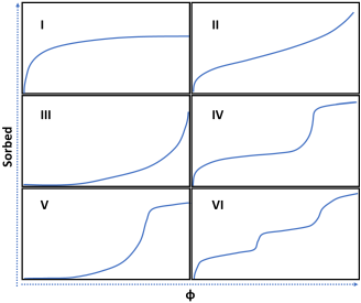
With enough A,B,C,D,E... parameters the master equation can replicate any isotherm, but loses meaning. An alternative is to make an approximation that the system is the combination of a simple curve and one or more mth order effects giving cooperative clustering and sigmoidal curves. There are 3 cases defined by IUPAC, Type IV, Type V,Type VI. If you have obvious multiple steps, choose Type VI from the start, and obtain the 8 parameters. Types IV and V have similar shapes, so how to choose between them? Because Type V has 4 parameters, if the fit is OK then use it, otherwise go to Type IV and gain the benefit of 5 parameters. The equations used involve the scaling constants N, in mol/kg with the other parameters being dimensionless:

Type IV

`"〈"n_2"〉"=N_a(A_1a_2)/(1+A_1a_2)+N_b(mA_ma_2^m)/(1+A_ma_2^m)`

Note that although you can fit this equation directly, it is difficult to get to the optimum. The app fits to the parameter `ln(A_m)/m` and uses information from the data such as the height of the cooperative step, and the position and gradient of the steepest gradient of the step. Doing this, the fitting starts with good estimates so is faster and more reliable.

Type V

`"〈"n_2"〉"=N(A_1a_2+mA_ma_2^m)/(1+A_1a_2+A_ma_2^m)`

Type VI and Type VI-like

IUPAC define Type VI as "layer-by-layer adsorption on a highly uniform nonporous surface". But it is common to use Type VI for multi-step sorption on porous surfaces - rarely are they called "Type VI-like". The equation is equally valid for both types as it makes no assumptions about the reasons for the multiple steps.

`"〈"n_2"〉"=N_a(A_1a_2)/(1+A_1a_2)+N_b(mA_ma_2^m)/(1+A_ma_2^m)+N_c(nA_na_2^n)/(1+A_na_2^n)`

The key things to look for are the m values. If they are small (<~5) then it's saying that not much cooperative clustering is taking place, when they are large (>~8) then that's a strong sign of such clustering. At the same time, large peaks in G22 are a good indication of strong cooperative clustering that coincides with the sort of sigmoidal curve for which the approach is best suited.

Analysis shows that fit quality can be similar for multiple pairs of Am and m values. This is partly a numerics issue and partly a data quality issue. If m is super-important then more data around the step is required to pin it down. But remember that m is intended to capture the broad essence of cluster sizes which will, in any case, cover a range of sizes, so it might not be worth the effort to obtain a more precise value.

Note that you can get quite good fits to most "normal" isotherms using these method but you are strongly advised not to use them - the standard theory is assumption free, while this theory is really only valid for the cases of strong clustering.

1

Seishi Shimizu and Nobuyuki Matubayasi, Sorption: A Statistical Thermodynamic Fluctuation Theory, Langmuir 2021, 37, 24, 7380–7391

2

Kaja Harton, Steven Abbott, Nobuyuki Matubayasi, Seishi Shimizu, Sorption isotherms: visualizing molecular interactions in preparation

3

Seishi Shimizu and Nobuyuki Matubayasi, Cooperative Sorption on Porous Materials, Langmuir 2021, 37, 34, 10279–10290

4

Olivia P. L. Dalby, Nobuyuki Matubayasi, and Seishi Shimizu, Cooperative Sorption on Heterogeneous Surfaces, xxx

5

M. Peleg, Models of Sigmoid Equilibrium Moisture Sorption Isotherms With and Without the Monolayer Hypothesis, Food Eng. Rev., 2020, 12, 1–13