Peel-Tack
Quick Start
The Peel test has been hard to link to the Probe Tack test. Here we implement an approach1 from the Ciccotti/Creton team at ESPCI in Paris to bring them together via core materials properties.
Credits
Prof Matteo Ciccotti kindly guided me through the task of appifying their theory.
Peel-Tack
                            //One universal basic required here to get things going once loaded
window.onload = function () {
    //restoreDefaultValues(); //Un-comment this if you want to start with defaults
    Main();
};
//Any global variables go here


//Main is hard wired as THE place to start calculating when input changes
//It does no calculations itself, it merely sets them up, sends off variables, gets results and, if necessary, plots them.
function Main() {
    saveSettings();

    //Send all the inputs as a structured object
    //If you need to convert to, say, SI units, do it here!
    const inputs = {
        a0: sliders.Slideh.value * 1e-6, //μm to m
        Bh: sliders.SlideBh.value * 1e-6, //μm to m
        BE: sliders.SlideBE.value * 1e9, //GPa to Pa
        F: sliders.SlideF.value,
        V: sliders.SlideV.value * 1e-3, //mm/s to m/s
        lx: sliders.Slidelx.value * 1e-3, //mm to m
    }

    //Send inputs off to CalcIt where the names are instantly available
    //Get all the resonses as an object, result
    const result = CalcIt(inputs)

    //Set all the text box outputs
    document.getElementById('af').value = result.af
    document.getElementById('erp').value = result.erp
    document.getElementById('edot').value = result.edot
    document.getElementById('sigma').value = result.sigma
    document.getElementById('Gamma').value = result.Gamma
    document.getElementById('GammaTack').value = result.GammaTack

    //Do all relevant plots by calling plotIt - if there's no plot, nothing happens
    //plotIt is part of the app infrastructure in app.new.js
    if (result.plots) {
        for (let i = 0; i < result.plots.length; i++) {
            plotIt(result.plots[i], result.canvas[i]);
        }
    }

    //You might have some other stuff to do here, but for most apps that's it for CalcIt!
}

//Here's the app calculation
//The inputs are just the names provided - their order in the curly brackets is unimportant!
//By convention the input values are provided with the correct units within Main
function CalcIt({ a0, Bh, BE, F, V, lx }) {
    const theta = Math.PI / 2 //fixed 90deg
    let xmax = 0
    while (xmax < lx + 1e-5) { //Crude way to get reasonable steps in axes
        xmax += 0.1e-3
    }
    const xmaxd=Math.floor(xmax*10000)/10
    const xstep = xmax / 1000
    const Inertia = Math.pow(Bh, 3) / 12
    const r = Math.sqrt(BE * Inertia / F)
    let Tape = [], x = 0, y = 0, yp = 0, s = 0, af = 0
    let PPts = []
    for (let i = 0; i <= 9; i++) PPts[i] = new Array(0)
    const sstep = lx / 9
    let snext = sstep, scount = 0
    for (x = 0; x <= xmax; x += xstep) {
        if (x <= lx) {
            yp = theta * (1 + ((x - lx) / r - 0.5 * Math.exp((x - lx) / r) + Math.exp(-x / r) * (1 - 0.5 * Math.exp(-lx / r))) / (lx / r + Math.exp(-lx / r) - 1))
        } else {
            yp = theta * (1 + Math.exp(-x / r) * (1 - Math.cosh(lx / r)) / (lx / r + Math.exp(-lx / r) - 1))
        }
        //Increase curvature near and beyond peel point. This is a visual fix only
        if (x > 0.9*lx) yp*=1+(x-0.9*lx)/0.001
        yp = xstep * Math.tan(Math.min(yp,0.99*theta))
        y += yp
        s += Math.sqrt(xstep * xstep + yp * yp)
        if (s >= lx && af == 0) {
            af = Math.sqrt(Math.pow(s - x, 2) + Math.pow(a0 + y, 2))
        }
        if (s >= snext && scount < 9) {
            PPts[scount][0] = { x: x * 1e3, y: (y + a0) * 1e3 }
            PPts[scount][1] = { x: snext * 1e3, y: a0 }
            snext += sstep; scount++
        }
        Tape.push({ x: x * 1e3, y: (y + a0) * 1e3 })
    }
    const erp = (af - a0) / a0
    const edot=erp*V/lx
    const sigma = F/(af-a0)

    //Now the tack
    //The graph is illustrative only
    let Tack=[],Gtack=0,yv=0,yvl=0
    const deta=erp/100, pval=erp/30, pval2=2*pval, tval=erp/30, sigmas=0.2*a0*1e6/150*F/400, spike=Math.min(3,Math.max(1.2,3*F/300))
    for (i=0;i<1.1*erp;i+=deta){
        if (i= pval && i < pval2){
            yv=Math.max(spike*sigma*(pval2-i)/pval,sigma*(1-sigmas))
        }
        if (i >= pval2 && i < 0.9*erp){
            yv=sigma*(1-sigmas+2*sigmas*(i-pval2)/erp)
            yvl=yv
        }
        if (i >= 0.9*erp){
            yv=yvl*Math.exp((0.9*erp-i)/tval)
        }
        Tack.push({x:i,y:yv/1e6}) //Pa to MPa
        Gtack+=yv*deta
    }
    Gtack*=a0

    //Now set up all the graphing data detail by detail.
    const prmap = {
        plotData: [Tape, PPts[0], PPts[1], PPts[2], PPts[3], PPts[4], PPts[5], PPts[6], PPts[7], PPts[8], PPts[9]], //An array of 1 or more datasets
        lineLabels: [], //An array of labels for each dataset
        hideLegend: true, //Set to true if you don't want to see any labels/legnds.
        xLabel: "x&mm", //Label for the x axis, with an & to separate the units
        yLabel: "y&mm", //Label for the y axis, with an & to separate the units
        y2Label: null, //Label for the y2 axis, null if not needed
        yAxisL1R2: [], //Array to say which axis each dataset goes on. Blank=Left=1
        logX: false, //Is the x-axis in log form?
        xTicks: undefined, //We can define a tick function if we're being fancy
        logY: false, //Is the y-axis in log form?
        yTicks: undefined, //We can define a tick function if we're being fancy
        legendPosition: 'top', //Where we want the legend - top, bottom, left, right
        xMinMax: [0, xmaxd], //Set min and max, e.g. [-10,100], leave one or both blank for auto
        yMinMax: [0,xmaxd], //Set min and max, e.g. [-10,100], leave one or both blank for auto
        y2MinMax: [,], //Set min and max, e.g. [-10,100], leave one or both blank for auto
        xSigFigs: 'F2', //These are the sig figs for the Tooltip readout. A wide choice!
        ySigFigs: 'F2', //F for Fixed, P for Precision, E for Math.exponential
    };
    const prmap1 = {
        plotData: [Tack], //An array of 1 or more datasets
        lineLabels: [], //An array of labels for each dataset
        hideLegend: true, //Set to true if you don't want to see any labels/legnds.
        xLabel: "ε& ", //Label for the x axis, with an & to separate the units
        yLabel: "σ&MPa", //Label for the y axis, with an & to separate the units
        y2Label: null, //Label for the y2 axis, null if not needed
        yAxisL1R2: [], //Array to say which axis each dataset goes on. Blank=Left=1
        logX: false, //Is the x-axis in log form?
        xTicks: undefined, //We can define a tick function if we're being fancy
        logY: false, //Is the y-axis in log form?
        yTicks: undefined, //We can define a tick function if we're being fancy
        legendPosition: 'top', //Where we want the legend - top, bottom, left, right
        xMinMax: [0,], //Set min and max, e.g. [-10,100], leave one or both blank for auto
        yMinMax: [0,], //Set min and max, e.g. [-10,100], leave one or both blank for auto
        y2MinMax: [,], //Set min and max, e.g. [-10,100], leave one or both blank for auto
        xSigFigs: 'F2', //These are the sig figs for the Tooltip readout. A wide choice!
        ySigFigs: 'F2', //F for Fixed, P for Precision, E for Math.exponential
    };

    //Now we return everything - text boxes, plot and the name of the canvas, which is 'canvas' for a single plot

    return {
        af : (af*1e3).toFixed(2),
        erp: erp.toFixed(1),
        edot: edot.toFixed(2),
        sigma : (sigma/1e6).toFixed(1),
        Gamma : F.toFixed(0),
        GammaTack : Gtack.toFixed(0),
        plots: [prmap,prmap1],
        canvas: ['canvas','canvas1'],
    };

}
For PSAs the key parameter of interest is peel strength. But for PSA development the probe tack test has always been useful. The problem was that there was no obvious link between the physics and the values of the two types of test.
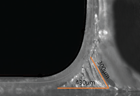
That changed with the work from the Ciccotti/Creton team at ESPCI. With a camera looking side-on at the peel they could see the shape and length, a, of the fibrils that appear as the peel front advances. From a precise mathematical fitting of the visual data to their peel theory they could work out the average stress, σpeel during extension of the fibrils and from the strain, εrupture at the point of peel failure they could work out the total energy dissipated during peel. If the length of the longest fibril is af and the starting thickness of the adhesive was a0 then `ε_(rupture)=(a_f-a_0)/a_0`.
In the image the PSA is being pulled with a force of 800 N/m. The longest fibre, length af, is 0.3mm and is attached to a point, LDebond 0.43mm from the peel front. The backing thickness was 40μm and the PSA was 60μm. This means that `ε_(rupture)=(300-60)/60=4`. These are the default values of the app and you see the simulated fibril structure is a reasonable match, though the calculation gives `a_f=0.29` so `ε_(rupture)=3.8`. However, the modulus of the backing tape is set to 1GPa instead of the real 3.6GPa to overcome a limitation in the app calculation, discussed below.
The team could also look at the average plateau stress during the probe tack test, along with the εrupture value which is remarkably close to that found during peel - provided both experiments were done at the same strain rate `dot ε_(peel)`.
An app approximation
Given the detailed mathematical analysis provided in the paper, it should have been possible to write an app that exactly carried out their calculations. Unfortunately it required a solver algorithm beyond my capabilities. So the app uses a simplified approximation taken from an earlier paper2 by the same team. The curvature of the tape is not as "sharp" as the real theory, but the approximation does a good job at conveying the general idea. If, as in the default settings, you reduce the modulus of the backing film, the simulation is able to partially overcome this limitation.
What is important for the calculations is not so much the shape of the curve, but the key parameters: adhesive thickness; base thickness & modulus; peel force and LDebond which is the length along the substrate from the start of peel to where the final fibril breaks. Plus, of course, the rate of peel to be matched to the rate of separation for tack in order to have the same strain rate.
To get LDebond from the experimental video requires the full curve fitting, for which the app is unsuited. But if you have a "good enough" estimate from your own measurements, this can be put into the app and the rest of the calculations are accurate.
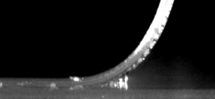
To build your intuitions, here are the data from a 20μm PSA on a 20μm backing film with a modulus of 2.9 GPa. LDebonding is 100μm so the fibrils are much closer to vertical and ε is ~1.7.
The tack curve
There is no pretence that the shape of the tack curve in the app is realistic. It is merely "representitive" of typical experimental curves. What is important is that it uses the σpeel as the mean tack stress value (some strain hardening is included for illustrative purposes) and εrupture values from the peel calculations (a starting peaks is included for illustrative purposes), so we are getting a good idea of what you would find if you compared the peel and tack data in a real experiment.
Work of debonding
The work of debonding is shown for peel, Γpeel and for tack Γtack. The peel value in J/m² is always exactly the same as the peel strength F in N/m provided as the input, because the internal calculations are based on F. The tack value is (as per the paper) the integral of the area under the peel curve: `Γ_(tack)=a_0int(σ(ε)δε)` where the integral is from 0 to εrupture. The resulting integral is usually a bit smaller than the peel value, as is found in the paper.
Acknowledgement
I am most grateful to Prof Ciccotti for patiently guiding me through the theory to help me create the app. All responsibility for errors is mine.
1Vivek Pandey, Antoine Fleury, Richard Villey, Costantino Creton and Matteo Ciccotti, Linking peel and tack performances of pressure sensitive adhesives, Soft Matter, 2020, 16, 3267
2Richard Villey, Pierre-Philippe Cortet, Costantino Creton, Matteo Ciccotti, In-situ measurement of the large strain response of the fibrillar debonding region during the steady peeling of pressure sensitive adhesives, Int J Fract (2017) 204:175–190