Chang Window
Quick Start
If you formulate a PSA into the wrong part of G' and G'' space then failure is guaranteed. So it is important to know where you need to be. This was defined by Dr Chang at Avery and later refined by others. The different "Chang Windows" for different PSA types need you to have the ability to measure G' and G'' at 0.01 and 100Hz. This is one of the many reasons why PSA formulators need access to good rheometers.
To use the app, just slide the sliders to define a "window" that covers the type of PSA you are formulting. By clicking the Modified or Full options you can see alternative views of the same basic principle.
The Chang Window
For a "typical" PSA Dahlquist tells us that G' should be <0.1MPa at ~1Hz. But how much less? And what value should it have at 0.01Hz or 100Hz? And what about G''? And what about different types of PSA for specialist applications? All these questions can be answered by looking through the Change Window, named after E.-P. Chang from the Avery Research Center.
First, we need to think of the timescales relevant to a PSA. Here is Chang's analysis of how G' will tend to vary at relevant frequencies:
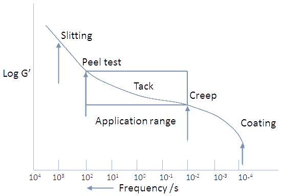
A PSA goes through a number of processes with very different characteristic frequencies, but the ones of interest to the application of a PSA are the ones shown in the "tack" area:
- Creep at ~0.01Hz
- Peel at ~100Hz
Now let us see the Chang Window in a choice of views, from basic to highly detailed:
Start with the Basic option. Along the X-axis is G'' in Pa. Along the Y-axis is G'. At any given measurement frequency a PSA will be a single point in that graph. But by defining a range of frequencies, from 0.01 to 100Hz each PSA will be represented by four points on the graph: (0.01, 0.01), (0.01, 100), (100,0.01) and (100,100), shown as a red rectangle superimposed onto the image.
Let us assume that you have measured your particular PSA and it's a beautifully middle-of-the-road material. The red rectangle will reside within the bigger rectangle (the "window") in the middle of the graph. As you change the G' and G'' values of your PSA the red rectangle might start to stray outside the classic PSA window. The labels in the quadrants outside the central Chang window give you some idea of the sort of PSA (or not!) your material would be. If, for example, you a cold temperature PSA you need to get the red rectangle into Quadrant 4. You really can design your PSA by numbers.
By selecting the "Modified" option you see the same Chang diagram but labelled rather differently according to Bartholomew's scheme. Finally, by selecting the "Full" option you see the Dahlquist criterion drawn along the top and a "tanδ=1" line drawn across the image. This should be a straight line but because the graphic is a rectangle, not a square, it has to be shown in that manner. Anything above and to the left of that line is tending to be "elastic" (and therefore a "normal" adhesive) and anything below and to the right of that line is tending to be "plastic" (and therefore a more typical PSA).
This whole scheme is devised for values of G' and G'' measured at 25°C. With WLF and a bit of ingenuity you can easily translate this scheme to other temperatures if, for example, you need a low temperature PSA.
Hopefully it is now clear why we had to take the journey from WLF through G-Values and Dahlquist to Chang. These basic concepts bring a large portion of PSA science into a single coherent system which has the double merits of being scientifically sound and applicable (as has been demonstrated many times) by the practical formulator.