AFM & Nanoindenters

In an ideal world we would all have SFA (Surface Force Apparatus) for measuring adhesion. They are the perfect tool because they measure the dependence of the key parameter, contact width (a), on applied force, F. It is a direct route from an SFA to working out the work of adhesion both in the loading and unloading curves.

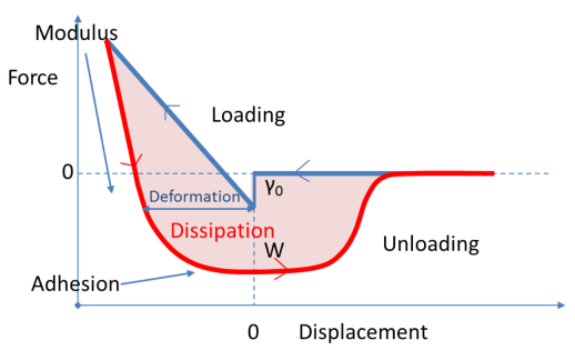Sadly, SFA are rather rare and have the reputation of being difficult to operate. On the other hand, AFM machines (small-scale) and nanoindenters (larger-scale) are relatively common and given a spherical probe (rather than the Berkovitch tip used for measuring modulus and hardness) one can obtain displacement versus force curves (as shown in the image) from which, with some extra effort, one can extract the work of adhesion. Experience suggests that a nanoindenter is a rather more robust methodology than an AFM for technical reasons connected to the way the forces are applied. What follows works well with a nanoindenter. The same theory should work OK for an AFM though the literature seems to imply greater difficulties in extracting accurate data because of cantiliver uncertainties and the very small radii of the probes which sample very small areas and have some issues with thicknesses of the coating being tested.

The literature makes it seem remarkably hard to extract meaningful JKR data from an indenter experiment. Fortunately the papers of Donna Ebenstein¹ cut through a lot of the complexities of generalised fits. If the radius, R, of the spherical tip is large (say 100μm or more)in comparison to the contact width and/or the indentation depth is small compared to the thickness of the sample, then the following analysis works well. (If (4RE*/3πγ)^0.333 >10 you don't need to use more sophisticated spherical punch geometries)In this simulation the desired outputs from a real experiment are actually inputs so you can see what the curves look like. In reality the loading and unloading curves are fitted to the appropriate equations in order to extract the key parameters.

Indentation v Force

In an ideal experiment the indentation is known exactly because the point of initial contact is known exactly. In practice there are large uncertainties about when the probe comes into contact (especially if there is an attractive "jump" of the probe to pull it into contact). So the value of the displacement δ at which contact is made, δ₀, has to be obtained by fitting. The equation relating displacement to contact width is known and can be calculated if the contact width at zero force, a₀ is known. But of course on a nanoindenter you have no way of knowing what this is. So this too has to be obtained by fitting. Finally, the analysis needs to know highest negative load, P_adh. In reality this point can be hard to identify because of sudden pull-off events, so it, too, has to be a fitting parameter.

The Ebenstein equation is:

δ-δ₀=a₀²/R((1+sqrt(1-P/P_adh))/2)^4/3- 2/3.a₀²/R((1+sqrt(1-P/P_adh))/2)^1/3

So, armed with δ₀, a₀ and P_adh from fitting to the data it is possible to calculate the work of adhesion from

γ = 0.667P_adh/(πR)

The curve also depends on reduced modulus, E_r calculated as:

E_r=-3RP_adh/a₀³

E_r depends on the moduli of the indenting sphere and of the sample. In many cases it is assumed that the sphere is infinitely hard compared to the sample - e.g. the sphere is made from glass. For practical adhesion we are usually interested in two relatively soft materials coming into contact (because we want intermingling or entanglement) so E_r is a mixture of the two moduli and their Poisson ratios, ν (assumed to be 0.3 unless you think that either is a rubber in which case it is 0.5):

1/E_r=(1-ν₁²)/E₁+(1-ν₂²)/E₂

Usually for adhesion the moduli are not of great interest, but if they are then you have to find a way to go from the reduced modulus to the individual values.

To explore the implications of all this, enter the pure surface energy γ_l for the loading curve. Add your estimates for δ₀ (default to 0), a₀ and P_adh, remembering that these would be outputs from the fitting of the curve that, for this model, is generated from all these inputs. Also add δ_max to show the upper bound of your indentation. Make sure that this is much less than the thickness of your sample.

The outputs are γ_u the work of adhesion (in unload) which might be a very high value if there is entanglement, the reduced modulus E_r, P_jump the jump in load when contact is made and δ_min where the load becomes the most negative. In a real experiment the curve continues below δ_min but it is hard to simulate convincingly and is not really usable for data fitting.

How do you use this technique in practice? If the aim is to understand adhesion between two materials of interest you have to make a (relatively thick) coating of one material onto a solid substrate such as glass - not too hard. But you also have to make a sphere of the second material and attach it to your probe. This is not easy! Or you have to find a way to coat a layer of your material onto a spherical probe and hope that it is sufficiently even to make the results meaningful. The point is that we have all spent our lives doing large amounts of work on adhesion with too little information. By putting some modest effort into refining this nanoindenter technique we may gain large amounts of understanding that will, in the long run, more than repay the effort put in to the measurements.