Hansen Solubility Parameters (HSP)

The ability of two polymers to intermingle or entangle depends, to a large extent, on how "like" they are. So all we need is an objective measure of likeness - or its opposite, the "distance" between two polymers. There is one scheme that does a good job at this and is described on this page. More details can be found on the Hansen Solubility site.

3 Parameters

Rather than rely on simplistic ideas of "hydrophilic/lipophilic" or "polar/non-polar" which are ill-defined terms, HSP use 3 parameters.

• δD is the "Dispersion" parameter which correlates with the polarisability of a molecule, which in turn correlates with refractive index and van der Waals forces. Molecules like methanol have few polarizable electrons so δD is low but aromatics like toluene have more polarizability and δD is higher. Similarly chlorinated solvents have a high δD because of the polarizable halogen electrons.
• δP is the "Polar" parameter and correlates with our intuitions about polar groups such as -OH or -C=O. Methanol, and acetone therefore have a relatively high δP and toluene a low value.
• δH is the "Hydrogen bonding" parameter and is obvious in terms of molecules such as methanol. However, molecules such acetone have a modest δH because the C=O is an acceptor for hydrogen donors.

Every solvent and polymer can be assigned its HSP. If the HSP values are similar then the solvent(s) and polymer(s) are compatible, if they are dissimilar then they are non-compatible. This encapsulates the intuition that "like attracts like". We can easily calculate how alike two molecules, 1 and 2, are from their HSP Distance defined as:

Distance²=4(δD1-δD2)²+(δP1-δP2)²+(δH1-δH2)²

Clearly if all 3 parameters for 1 and 2 are very close, then Distance is small and mutual solubility/compatibility is high. If one or more values differ greatly then the Distance is large and mutual solubility is low.

For those who are used to the Flory-Huggins χ parameter for thinking about polymer solubility, it is calculated via:

χ=MVol*Distance²/4RT

where MVol is the molar volume and RT is the usual gas constant times temperature term. For polymer-polymer intermingling (rather than complete mutual solubility which is hard to achieve) the χ parameter can be used to calculate the distance two polymers can reach across the interface, with a lower χ value giving a greater possibility of intermingling. In other words, the HSP Distance is a good guide to polymer intermingling even if (for those who know Painter-Coleman) they are a less good guide to polymer miscibility.

Applying HSP

The app lets you calculate some HSP distances between common polymers polymers. Simply select a pair and the HSP distance is calculated. Although it is well-known that most polymers (at high MWt) are immiscible, at an interface between them the distance that the polymer chains can intermingle can be significant - even for polymers that aren't very close. This makes the "diffusion" theory of adhesion much more likely (and, in fact, provable). The intermingle distance d is based on the "statistical bond length" (Kuhn length) which for simplicity here can be taken to be equivalent to 5 C-C bond lengths, i.e. 0.7nm. and is given by the Helfand formula:

d=b/(6χ)^0.5. The transformation of χ from Distance uses a value of 50000 for MVol of the polymers.

Solvent Blends

A blend of two solvents can often have better solubility properties (lower HSP Distance) than either of the individual solvents which might even be non-solvents for the target materials.

With this app you can try out these ideas. Choose a target polymer, then various pairs of solvents and vary their ratio till you get the best match (lowest HSP Distance or Ra):

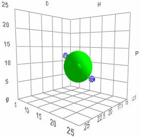When Charles first came up with his HSP scheme he saw that it made a surprising prediction. That two bad solvents (the blue dots in the image) on opposite sides of the HSP Sphere should produce an excellent solvent (green dot in the middle) when mixed 50:50. If his HSP ideas were wrong then mixing two bad solvents would create another bad solvent. When he did the test his ideas were confirmed - you really can make a good solvent from a mixture of bad ones.

This is probably the single most useful idea in the whole of HSP. It allows formulators amazing freedom to combine solvents that are attractive in terms of cost, safety, odour, volatility etc. but which are poor solvents for the specific system and create an excellent solvent blend. By being smart with the relative volatilities of the solvents it's possible to make mixes that deliberately crash out the solutes when evaporation starts (the best solvent is more volatile) or crash out one solute component (its best solvent is more volatile) or, alternatively, to make a super-smooth coating by ensuring that the best solvent for the critical component is the least volatile so keeps it in solution up to the last moment.