
Foam Flow
Quick Start
Using a "dam burst" or "L-box" test you can quickly get values for foam viscosity and yield stress.
With advanced simulations the whole flow can be modelled; in this development version we use some approximations that have proven more than adequate.
Credits
The app is part of the work of the LASTFIRE team working towards improved on-site knowledge of foam properties relevant to fighting fires.
Foam Flow
//One universal basic required here to get things going once loaded
window.onload = function () {
    //restoreDefaultValues(); //Un-comment this if you want to start with defaults
    Main();
};

//Main() is hard wired as THE place to start calculating when inputs change
//It does no calculations itself, it merely sets them up, sends off variables, gets results and, if necessary, plots them.
function Main() {
    //Save settings every time you calculate, so they're always ready on a reload
    saveSettings();

    //Send all the inputs as a structured object
    //If you need to convert to, say, SI units, do it here!
    const inputs = {
        H: sliders.SlideH.value / 100, //to m
        L: sliders.SlideL.value / 100, //to m
        S: sliders.SlideS.value,
        DStop: sliders.SlideDStop.value / 100, //to m
        t1: sliders.Slidet1.value,
        t2: sliders.Slidet2.value,
        t3: sliders.Slidet3.value,
        t4: sliders.Slidet4.value,
        Dt1: sliders.SlideDt1.value / 100, //to m
        Dt2: sliders.SlideDt2.value / 100, //to m
        Dt3: sliders.SlideDt3.value / 100, //to m
        Dt4: sliders.SlideDt4.value / 100, //to m
    };

    //Send inputs off to CalcIt where the names are instantly available
    //Get all the resonses as an object, result
    const result = CalcIt(inputs);

    //Set all the text box outputs
    document.getElementById('tau').value = result.tau;
    document.getElementById('eta').value = result.eta;
    document.getElementById('Error').value = result.err;
    document.getElementById('dtWrong').value = result.dtWrong;
    if (result.dtWrong.includes("wrong")) {
        document.getElementById('dtWrong').style.backgroundColor = "pink"
    } else {
        document.getElementById('dtWrong').style.backgroundColor = document.getElementById('eta').style.backgroundColor
    }
    if (result.plots) {
        for (let i = 0; i < result.plots.length; i++) {
            plotIt(result.plots[i], result.canvas[i]);
        }
    }
}

//Here's the app calculation
//The inputs are just the names provided - their order in the curly brackets is unimportant!
//By convention the input values are provided with the correct units within Main
function CalcIt({ H, L, S, DStop, t1, t2, t3, t4, Dt1, Dt2, Dt3, Dt4 }) {

    const dsWrong = (Dt1 > Dt2 || Dt2 > Dt3 || Dt3 > Dt4 || Dt4 > DStop)
    const tsWrong = (t1 >= t2 || t2 >= t3 || t3 >= t4)

    let FPts = [], t1Pts=[],t2Pts=[],t3Pts=[],t4Pts=[],aPts=[]
     const rhog = 9.81 * 1000 / S

    DStop += L //We measure from where we removed the dam, but the calc is from the start
    const P3 = Math.pow(3, 2 / 3)
    let B = Math.pow(P3 / (2 * DStop / L), 3), tpow = 0.5, tpp = 1
    const tau = B * rhog * H * H / L

    let tinc = 0.001, x = 0, preFactor, minErr = 999999, err
    const tInertia = 1
    eta = 1
    DStop -= L //Back to our definition
    //We don't know eta so we need to find the best fit to our data, varying eta from 0.1 to 15 Pa.s
    for (e = 0.5; e <= 15; e += 0.1) {
        preFactor = 0.2845 * Math.pow(H, 3 / 2) * Math.sqrt(rhog / e)
        x = 0, tinc = 0.001, tpp = 1
        let tS1 = tS2 = tS3 = tS4 = 0
        for (let t = 0.001; t <= 2 * t4; t += tinc) {
            // There are a number of theories out there, but this approximation works OK
            tpow = 0.5 - 0.3 * Math.pow(Math.min(1, x / DStop), 0.5)
            x = preFactor * Math.pow(t, tpow)
            if (tS1 == 0 && x > Dt1) { tS1 = t }
            if (tS2 == 0 && x > Dt2) { tS2 = t }
            if (tS3 == 0 && x > Dt3) { tS3 = t }
            if (tS4 == 0 && x > Dt4) { tS4 = t }
            if (t > 0.05) tinc = 0.01
            if (t > 1) tinc = 0.1
        }
        err = Math.pow((tS1 - t1), 2) + Math.pow((tS2 - t2), 2) + Math.pow((tS3 - t3), 2) + Math.pow((tS4 - t4), 2)
        if (err < minErr) { minErr = err; eta = e }
    }
    x = 0; tinc = 0.001, tpp = 1
    //Use our optimized eta
    preFactor = 0.2845 * Math.pow(H, 3 / 2) * Math.sqrt(rhog / eta)
    for (let t = 0.001; t <= t4+0.9*tinc; t += tinc) {
        // Using the same theory with our optimized eta
        tpow = 0.5 - 0.3 * Math.pow(Math.min(1, x / DStop), 0.5)
        x = preFactor * Math.pow(t, tpow)
        if (x > DStop) break
        FPts.push({ x: t, y: x * 100 }) //to cm
        if (t > 0.05) tinc = 0.01
        if (t > 1) tinc = 0.1
    }
    t1Pts.push({x:t1,y:0},{x:t1,y:Dt1*100})
    t2Pts.push({x:t2,y:0},{x:t2,y:Dt2*100})
    t3Pts.push({x:t3,y:0},{x:t3,y:Dt3*100})
    t4Pts.push({x:t4,y:0},{x:t4,y:Dt4*100})
    aPts.push({x:0,y:DStop*100},{x:t4,y:DStop*100})
    //Now we return everything - text boxes, plot and the name of the canvas, which is 'canvas' for a single plot
    const prmap = {
        plotData: [FPts,t1Pts,t2Pts,t3Pts,t4Pts,aPts], //An array of 1 or more datasets
        lineLabels: ["Flow"], //An array of labels for each dataset
        hideLegend: true,
        colors:['#edc240',"skyblue","skyblue","skyblue","skyblue","skyblue"],
        dottedLine: [false,true,true,true,true,true],
        xLabel: 't&s', //Label for the x axis, with an & to separate the units
        yLabel: "D&cm", //Label for the y axis, with an & to separate the units
        y2Label: null, //Label for the y2 axis, null if not needed
        yAxisL1R2: [], //Array to say which axis each dataset goes on. Blank=Left=1
        logX: false, //Is the x-axis in log form?
        xTicks: undefined, //We can define a tick function if we're being fancy
        logY: false, //Is the y-axis in log form?
        yTicks: undefined, //We can define a tick function if we're being fancy
        legendPosition: 'top', //Where we want the legend - top, bottom, left, right
        xMinMax: [,], //Set min and max, e.g. [-10,100], leave one or both blank for auto
        yMinMax: [,], //Set min and max, e.g. [-10,100], leave one or both blank for auto
        y2MinMax: [,], //Set min and max, e.g. [-10,100], leave one or both blank for auto
        xSigFigs: 'P3', //These are the sig figs for the Tooltip readout. A wide choice!
        ySigFigs: 'P3', //F for Fixed, P for Precision, E for exponential
    }
    return {
        tau: (tau).toFixed(2),
        eta: eta.toPrecision(2),
        dtWrong: (dsWrong ? "D wrong" : "D  OK") + (tsWrong ? ", t wrong" : ", t  OK"),
        err: minErr.toPrecision(3),
        plots: [prmap],
        canvas: ['canvas'],
    };
}
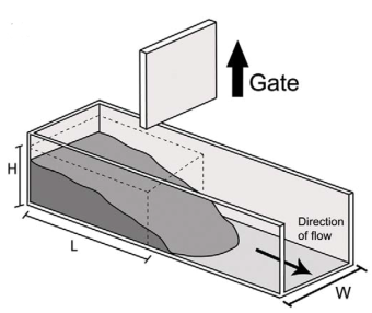 In the dam burst or L-box test you fill a partition of length L with foam to height H (the width W is not important, other than for edge effects which can be ignored if the box is pre-wetted). At time t=0 you pull up the gate and using a video camera with a clear view of the scale inscribed on the bottom of the box you see that the foam, of density ρ=1/S (S=Expansion) and viscosity η flows a distance D in time t given, in the early stages, by the following formula where n=0.5.
`D=0.285H^1.5((ρg.t)/η)^n`
However, given a yield stress τ, the foam will stop flowing at a distance Dstop that depends on B the Bingham number given by:
`B=(τL)/(ρgH^2)`
If B<1/3, which should be the case for fire foams, then the flow stops when
`D_"stop"=1/(B^0.333)`
Because Dstop is known experimentally (see below) the app can then calculate τ. But deriving η requires fitting to the whole flow curve for which there is no agreed simple equation. So we use the same flow equation for D but the power n decreases steadily as D approaches Dstop.
From test data to parameters
You can press Stop on your video playback after a set of fixed times such as 2, 4, 8, 16 seconds (or whatever makes sense with your real data). At each point you record how far the flow has come, as well as Dstop after a suitably long time (there's some judgement here as the flow becomes very slow, but it's not necessary to be super-precise).
Now enter your times and the respective D values, they are shown as vertical dotted lines. Because of the slow approach to Dstop the visual check of your value, as a horizontal dotted line, is helpful. There is a check made that all times and D values increase from left to right so you can't accidentally create a very bad setting. It might be easier in future versions to be able to type values as strings into text boxes, but during this development phase the sliders are convenient.
Once you've entered your values you get values for τ and η. As you will be uncertain about some of your measurements, gently slide the values and check the Error value. Don't worry about its absolute value, just tweak the sliders to minimize it for this specific setup. You quickly converge on a self-consistent dataset. The dotted lines are also good for seeing if the curve makes sense.
Optimal H, L and W and box length
Defaults of H=10 and L=10 are a good starting point, but if it's possible give yourself the flexibility in the design of H=10 to 20 and L=5 to 15, with larger values used for stiffer/lighter foams. The box width, W, is not important above, say, 20cm as the edge effects are small if the box has been pre-wetted. The trick with pre-wetting is to get a uniform thin layer of water (helped with a bit of surfactant) on the walls and base of the channel, as well as on the inner side of the dam, to reduce the effects of swift removal. Any significant amount on the base will shift the yield from the foam/box to foam/water which is much lower - most foams flow freely on water.
A box length of ~60cm seems to work well and scale marks every 1 cm provide enough accuracy, given that the flow front is not perfectly straight.
Are the results accurate?
The experimental measurements have uncertainties, the foam itself might be changing during the measurement, the theory is approximate and even the idea of there being an exact value for a yield stress is controversial. So, no, the results are not "accurate". But are they repeatable and useful? Yes! The method, along with the bubble radius measurement, gives us a way to capture core differences between foams and relate them to end performance. The test is meant for the real world and can be done just about anywhere where there's some flat ground, some shielding from the worst of the wind and rain and a way to get some fresh foam from the nozzle into the dam area.
The theory is taken from Angelo Castruccio, A.C. Rust, R.S.J. Sparks, Rheology and flow of crystal-bearing lavas: Insights from analogue gravity currents, Earth and Planetary Science Letters 297 (2010) 471–480, showing that lava flows and fire foams follow the same physics. That paper in turn is based on the full analysis in N.J. Balmforth, R.V. Craster, P. Perona, A.C. Rust, R. Sassi, Viscoplastic dam breaks and the Bostwick consistometer, J. Non-Newtonian Fluid Mech. 142 (2007) 63–78. Another name for the dam burst test is a Bostwick consistometer.