Dynamic Surface Tension
Quick Start
DST is important in many industries (e.g. coating, spraying) were fresh surface is created and a low surface tension is required. There are two approaches to the topic. The one here looks at DST as a general phenomenon, and allows you to build up your intuitions about what is going on. The second, in DST Choice, looks at the phenomenon in a more real-world approach. I personally find both to be useful.
This app uses the approach of the great Rosen, so it deserves some careful reading.
DST
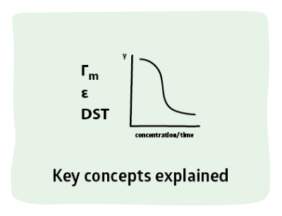 When a fresh water/air interface is created in a surfactant solution the surface tension is assumed to be 72mN/m. As the surfactant comes to the surface the Surface Tension (ST) drops or, it comes to the same thing, the Surface Pressure (SP = Original ST - ST at time t) rises.
There are many ways to approach the problem but the most useful is that of Rosen. Although the equation below has no obvious link to theory it works well for most cases and is far more insightful than approaches which focus on the details of just one aspect of the curve. In a Log plot the shape of the curve is sigmoidal with a slow Induction period up to a time ti followed by a rapid reduction of ST characterised by a time t* before turning into a slow approach to the equilibrium value γc. For some surfactants the value reached after a few seconds is ~5 mN/m higher than the equilibrium value. In this simplified version no distinction is made between this short-term plateau value and the longer-term equilibrium value.
The rapid reduction is governed by a power n according to the formula and nomenclature of Rosen
`γ_t=γ_c+(γ_0-γ_c)/[1+(t/(t"*"))^n]`
For a given surfactant at a given concentration the equilibrium value γc is known and it is possible to fit the experimental data to find t* and n
Simulating a surfactant
Simply enter values for γc, t* and n and the App calculates either ST or SP depending on your selected option. The data can be viewed in log, linear, square root or inverse square root form depending on your interest. The starting time t0 and ending time tMax can also be chosen
Diffusion Coefficient
The diffusion coefficient of the surfactant controls the speed of the induction phase. By plotting SP v square root time up to the end of the initiation phase it is possible to calculate the (apparent) diffusion coefficient. The word "apparent" is used because in principle the diffusion to the surface can be different from diffusion in the bulk, but in most situations the differences are not large (even in cases where there is proven "mixed mode" diffusion the changes in apparent coefficient are rather small). Rosen was able to show that the induction time can be calculated via:
`log10(t_i)=log10(t"*")-1/n`
Using the assumption that the induction process makes sense over a decade of time, the plot of square root time v SP is made from ti/10 to ti. Using the Slope (from a least squares fit) and knowing the bulk molar surfactant concentration C0 (entered via a number and exponential, so 3.2E^-4 would be entered as 3.2 and -4) and assuming T=25degC so that RT~2479 the diffusion coefficient is calculated as:
`D=π((Slope)/(C_0 2RT))^2`
For typical surfactants, D is in the order of 0.5-2*10^-6cm²/s. ti and D are always calculated. But when the Induction option is chosen the graph shows the plot and the least squares fit. Of course there are many assumptions in this chain of reasoning and the modeller is only a way of illustrating broad trends in dynamic surface tension. Ideally, for example, the induction curve should extrapolate back to 0 at t=0 but in practice this often doesn't happen and only the slope is used.
Experts will note that there is a square root time dependence when the system is approaching equilibrium. This requires a different fitting formula and the apparent diffusion coefficient is often a factor of 5 to 50 lower than the real diffusion coefficient. Although the complexities of this period seem to be of great interest to theoreticians most users have little interest in whether the ST goes from 41 to 40 or 41 to 39 over another few seconds because generally the interest is what is happening at short timescales where rapid diffusion helps the induction phase.
Changing Concentration
It is assumed that the input t* and n values are from data at a given surfactant concentration. The t* value depends, of course, on surfactant concentration - the higher the concentration, the faster the ST or SP reaches the equilibrium value. The dependency is given by a general formula:
`log(t"*"")=a.log(γ_(max)/C)+b`
where a is the Log.Fact., b is the Lin.Fact., C is the molar concentration and Γmax is the maximum surface (excess) concentration of the surfactant.
In this simple modeller, if the Conc.Mode option is selected then Γmax is calculated from the given t* value at the given C0 value. This then allows t* (and ti and D) to be calculated for each new value of the concentration, C1.
Of course, as the concentration increases, the equilibrium value will reduce until the CMC is reached. Using the rule of thumb (or, if you prefer, using an approximation to the Langmuir isotherm) that a factor of 10 reduction in surfactant concentration below the CMC results in an increase of ST of 20 mN/m it is possible to use the given equilibrium ST and the CMC input values (shown as C* for layout reasons) to estimate the ST at the CMC (if C0 < CMC) and thus to estimate the equilibrium ST at C1.
Experts will note the many assumptions behind these calculations, but overall the trends are in the right direction - and if someone can suggest a better way to do the calculations I will be happy to use it.
No CMC Special Effects
It seems reasonable to assume that above the CMC the rules might change, so the above formulae would need to change to accommodate more than just the fact that the equilibrium value becomes a constant at and above the CMC. However there are lots of data to show that nothing special happens at the CMC in terms of DST so the approximations above are surprisingly robust. To put it another way, the fact that excess surfactant exists in micelles has no obvious effect on t* and ti.
n and t* dependencies
In the absence of any other data, a value of 1 for n is reasonable. Values for standard surfactants seem to vary between 0.5 and 1.5. The general trend is that the more hydrophobic the surfactant (e.g. longer chain or shorter EO number for ethoxylate) the larger the value of n. Branched chains tend to reduce n. For ionics, increase ionic strength also increase n. t* follows the trends in n. Increasing n means faster equilibration and increasing t* means slower equilibration so the fact that they move in the same direction might seem to imply that they balance each other out. Two factors modify this impression. First, increases in n tend to go with decreases in the equilibrium ST so the absolute ST will decrease faster with higher n. Second, the t* effect is slightly complicated and you might get faster initial reductions and slower long-time reductions (or vice versa). Happily, the model lets you explore all these factors "live".