Contact Angle via Sessile Drop
Quick Start
Measuring contact angle is easy with a fancy device. But if you've just got a smartphone, some lighting and can place a drop carefully onto the level surface, you can load the captured image into the app to get a good-enough value via some simple fitting.
Credits
The Young-Laplace algorithm used to fit the drop shape is the one used in the Young-Laplace app.
Contact Angle from Sessile Drop
'use strict'
//One universal basic required here to get things going once loaded
let image, edge, edgemin, edgemax, imgWidth, imgHeight, context, imageData, oldImageData, oldAngle = 0, xMin,xMax,yMin,yMax

window.onload = function () {
    //restoreDefaultValues(); //Un-comment this if you want to start with defaults
    document.getElementById('Load').addEventListener('click', clearOldName, false);
    document.getElementById('Load').addEventListener('change', handleFileSelect, false);

    loadAndDrawImage("img/10ul H2O on PTFE Exemplar.png")
    //loadAndDrawImage("img/Test2.jpg")
    //Main();
};

document.getElementById('SlidersAsText').addEventListener('change', (e) => {
    Object.values(sliders).forEach(slider => slider.setTextMode(e.target.checked));
});


//Main is hard wired as THE place to start calculating when input changes
//It does no calculations itself, it merely sets them up, sends off variables, gets results and, if necessary, plots them.
function Main() {
    saveSettings();
    //Send all the inputs as a structured object
    //If you need to convert to, say, SI units, do it here!
    const inputs = {
        h: sliders.Slideh.value / 1e3,
        b: sliders.Slideb.value / 1e3,
        delta: sliders.Slidedelta.value * 1e3,
        sigma: sliders.Slidesigma.value / 1e3,
        mm: sliders.Slidemm.value,
        Base: sliders.SlideBase.value,
        Xoffs: sliders.SlideXoffs.value,
        Xrange: sliders.SlideXrange.value,
        Yrange: sliders.SlideYrange.value,
       Angle: sliders.SlideAngle.value * Math.PI / 180, //Deg to Rad
    }
    //These are convenient as direct global variables
        xMin = sliders.SlidexMin.value/100 //From %
        xMax = sliders.SlidexMax.value/100 //From %
        yMin = sliders.SlideyMin.value/100 //From %
        yMax = sliders.SlideyMax.value/100 //From %

    //Send inputs off to CalcIt where the names are instantly available
    //Get all the resonses as an object, result
    const result = CalcIt(inputs)

    //Set all the text box outputs
    document.getElementById('Volume').value = result.Volume
    document.getElementById('Width').value = result.Width
    document.getElementById('CA').value = result.CA

    //Do all relevant plots by calling plotIt - if there's no plot, nothing happens
    //plotIt is part of the app infrastructure in app.new.js
    if (result.plots) {
        for (let i = 0; i < result.plots.length; i++) {
            plotIt(result.plots[i], result.canvas[i]);
        }
    }

    //You might have some other stuff to do here, but for most apps that's it for CalcIt!
}

//Here's the app calculation
//The inputs are just the names provided - their order in the curly brackets is unimportant!
//By convention the input values are provided with the correct units within Main
function CalcIt({ h, b, delta, sigma, mm, Base, Xoffs, Xrange, Yrange, Angle }) {
    if (oldImageData != null) DoStuff(Base, mm, Angle)
    let tmp = [], DPlot = [], EPlot = [], z = h, x = 0, phi = 0, Volume = 0, R = 2 * b, dz = 0
    const phiinc = 0.001, pi = Math.PI, g = 9.81, dgs = delta * g / sigma
    let maxWidth = 0, cWidth = 0
    for (phi = 0; phi < pi; phi += phiinc) {
        tmp.push({ x: x * 1e3, y: z * 1e3 })
        x += R * Math.cos(phi) * phiinc
        maxWidth = Math.max(x, maxWidth)
        dz = R * Math.sin(phi) * phiinc
        z -= dz
        R = 1 / (dgs * (h - z) + 2 / b - Math.sin(phi) / x)
        Volume += pi * dz * x * x
        if (z <= 0) break
        cWidth = x //This will contain the last width before z=0
    }
    const CA = phi * 180 / Math.PI
    const tl = tmp.length - 1
    for (let i = 0; i <= tl; i++) {
        DPlot.push({ x: -tmp[tl - i].x, y: tmp[tl - i].y })
    }
    for (let i = 0; i < tmp.length; i++) {
        DPlot.push({ x: tmp[i].x, y: tmp[i].y })
    }
    //Now plot the edge, suitable scales/centered
    if (edge) {
        const mmW = mm / imgWidth
        const correction = mm / 2 + (edgemin * mmW - edgemax * mmW) / 2
        for (let i = 0; i < edge.length; i++) {
            if (edge[i].x > imgWidth*xMin && edge[i].x < imgWidth*xMax && edge[i].y > imgHeight*yMin && edge[i].y < imgHeight*yMax)  EPlot.push({ x: edge[i].x * mmW - correction + Xoffs, y: Math.max(0, -Base + (imgHeight - edge[i].y) * mmW) })
        }
    }
    //Now set up all the graphing data detail by detail.
    let plotData = [DPlot, EPlot]
    let lineLabels = ["Calculated", "Edge"] //An array of labels for each dataset
    let xMM = [], yMM = []
    if (document.getElementById("Magnify").checked) {
        xMM.push(-Xrange); xMM.push(Xrange)
        yMM.push(h * 1e3); yMM.push(h * 1e3 - Yrange)
    } else {
        // xMM.push(-Math.ceil(2*maxWidth * 1000)/2);xMM.push(Math.ceil(2*maxWidth * 1000)/2)
        // yMM.push();yMM.push()
    }
    const prmap = {
        plotData: plotData,
        lineLabels: lineLabels,
        hideLegend: true,
        xLabel: "x& mm", //Label for the x axis, with an & to separate the units
        yLabel: "z& mm", //Label for the y axis, with an & to separate the units
        y2Label: undefined, //Label for the y2 axis, null if not needed
        yAxisL1R2: [], //Array to say which axis each dataset goes on. Blank=Left=1
        logX: false, //Is the x-axis in log form?
        xTicks: undefined, //We can define a tick function if we're being fancy
        logY: false, //Is the y-axis in log form?
        yTicks: undefined, //We can define a tick function if we're being fancy
        legendPosition: 'top', //Where we want the legend - top, bottom, left, right
        xMinMax: xMM, //Set min and max, e.g. [-10,100], leave one or both blank for auto
        yMinMax: yMM, //Set min and max, e.g. [-10,100], leave one or both blank for auto
        y2MinMax: [,], //Set min and max, e.g. [-10,100], leave one or both blank for auto
        xSigFigs: 'F2', //These are the sig figs for the Tooltip readout. A wide choice!
        ySigFigs: 'F1', //F for Fixed, P for Precision, E for exponential
    };

    //Now we return everything - text boxes, plot and the name of the canvas, which is 'canvas' for a single plot

    return {
        Volume: (Volume * 1e9).toFixed(1),
        Width: (2 * cWidth * 1000).toFixed(1), // +" : " + (2*maxWidth * 1000).toFixed(1),
        CA: CA.toFixed(1),
        plots: [prmap],
        canvas: ['canvas'],
    };

}

function loadAndDrawImage(url) {
    // Create an image object. This is not attached to the DOM and is not part of the page.
    oldImageData = null
    image = new Image();

    // When the image has loaded, draw it to the canvas
    image.onload = function () {
        DoStuff(0, 0, 0)
        Main()
    }
    // Now set the source of the image that we want to load
    image.src = url;
}
function DoStuff(Base, mm, Angle) {

    canvas1.width = image.width;
    canvas1.height = image.height;
    document.getElementById("canvas1").style.cursor = "crosshair"

    context = canvas1.getContext("2d", { willReadFrequently: true });
    context.translate(canvas1.width / 2, canvas1.height / 2)
    context.rotate(Angle)
    context.translate(-canvas1.width / 2, -canvas1.height / 2)
    //context.filter = 'blur('+Smoothing+'px)';
    context.drawImage(image, 0, 0);
    if (oldImageData == null || oldAngle != Angle){ //|| oldSmoothing != Smoothing) {
        imageData = context.getImageData(0, 0, canvas1.width, canvas1.height);
        oldImageData = new Uint8ClampedArray(imageData.data)
    } else {
        imageData.data.set(oldImageData)
    }
    if (Base == 0 && mm == 0 && Angle == 0) return

    oldAngle = Angle//;oldSmoothing=Smoothing
    const data = imageData.data;
    const xSize = imageData.width, ySize = imageData.height
    imgWidth = xSize; imgHeight = ySize
    const threshold = sliders.Slidethreshold.value * 3
    let x, y, pos
    for (y = 1; y < ySize - 1; y++) {
        for (x = 0; x < xSize - 0; x++) {
            pos = (y * xSize + x) * 4;
            if (data[pos] + data[pos + 1] + data[pos + 2] > threshold) {
                data[pos] = 255; data[pos + 1] = 255; data[pos + 2] = 255
            }
            else {
                data[pos] = 0; data[pos + 1] = 0; data[pos + 2] = 0
            }
        }
    }
    edge = [], edgemin = xSize; edgemax = 0;
    for (y = 1; y < ySize; y++) {
        for (x = 1; x < xSize; x++) {
            pos = (y * xSize + x) * 4;
            if (data[pos - 4] > data[pos]) {
                edge.push({ x: x, y: y + 1 })
                if (y >= ySize*yMin && y <= ySize*yMax && x >= xSize*xMin && x <= xSize*xMax) edgemin = Math.min(edgemin, x)
                     for (let yy = Math.max(y-8,0); yy < Math.min(ySize-1,y + 8); yy++) {
                    for (let xx = Math.max(x-8,0); xx < Math.min(xSize-1,x + 8); xx++) {
                        pos = (yy * xSize + xx) * 4
                         data[pos + 1] = 255; data[pos + 2] = 255
                    }
                }
                break
            }
        }
    }
    for (y = ySize; y > 0; y--) {
        for (x = xSize - 1; x > 0; x--) {
            pos = (y * xSize + x) * 4;
            if (data[pos] > data[pos - 4]) {
                edge.push({ x: x, y: y + 1 })
                if (y >= ySize*yMin && y <= ySize*yMax && x >= xSize*xMin && x <= xSize*xMax) edgemax = Math.max(edgemax, x)
                for (let yy = Math.max(y-0,0); yy < Math.min(ySize-1,y + 8); yy++) {
                    for (let xx = Math.max(x-8,0); xx < Math.min(xSize-1,x + 0); xx++) {
                        pos = (yy * xSize + xx) * 4
                         data[pos + 1] = 255; data[pos + 2] = 0
                    }
                }
                break
            }
        }
    }

    edgemax = xSize - edgemax
    if (!document.getElementById("Original").checked) context.putImageData(imageData, 0, 0)

    if (yMin > 0 || yMax < 1) {
        context.beginPath();
        context.strokeStyle = "magenta"
        context.lineWidth = 3
        context.moveTo(0, canvas1.height * yMin);
        context.lineTo(canvas1.width, canvas1.height * yMin);
        context.stroke();
        context.moveTo(0, canvas1.height * yMax);
        context.lineTo(canvas1.width, canvas1.height * yMax);
        context.stroke();
    }
    if (xMin > 0 || xMax < 1) {
        context.beginPath();
        context.strokeStyle = "magenta"
        context.lineWidth = 3
        context.moveTo(canvas1.width * xMin, 0);
        context.lineTo(canvas1.width * xMin, canvas1.height);
        context.stroke();
        context.moveTo(canvas1.width * xMax,0);
        context.lineTo(canvas1.width * xMax,canvas1.height);
        context.stroke();
    }

}
function clearOldName() { //This is needed because otherwise you can't re-load the same file name!
    document.getElementById('Load').value = ""
}
function handleFileSelect(evt) {
    var f = evt.target.files[0];
    if (f) {
        if (f.type !== '' && !f.type.match('image.*')) {
            return;
        }
        // The URL API is vendor prefixed in Chrome
        window.URL = window.URL || window.webkitURL;

        // Create a data URL from the image file
        var imageURL = window.URL.createObjectURL(f);

        loadAndDrawImage(imageURL);
    }
}
The 4 problems
There are 4 problems for measuring contact angle:
- Placing a controlled drop of fluid onto the surface which is perfectly level.
- Capturing a well-lit, high-contrast image of the drop and knowing the width, in mm, of the whole image.
- Getting rid of artefacts in the image to make fitting easier.
- Fitting the drop shape in order to extract the contact angle.
A wonderful 3D-printed device is under development for tasks 1 and 2 and all relevant parts/files will be provided once we've finished the final debugging. The trick is to use a modern, high quality, low cost ($50) digital microscope. But for now, let's assume you have a good-enough image.
You need to input three pieces of real data:
- ρ: The density of your probe liquid. As this is often water, the default value is 1
- σ:The surface tension of your liquid - defaulting to 72 mN/m for water
- Image Width: The width of the full image, which defines the scale used to compare calculated to real drop shape
Now there are 5 fitting parameters (the Threshold value is discussed below). The first 2 are all about the drop, the others are about aligning/adjusting the image to allow you to get reliable values for the first 2. Perfectly-lit drops on perfect substrates shouldn't need extra adjustments, but images of drops on real substrates with real lighting need plenty of help from the adjustments:
- h: The height of the drop from interface to heighest point.
- b: This is the radius of curvature of the drop at its highest point.
- Base offset: This allows you to define where in the image the drop starts. It's surprisingly hard to pinpoint the drop/substrate interface.
- X-offset: This allows you to shift the fitted image left-right to fix symmetry issues.
- Rotation: This allows you to fix problems with (slightly) tilted images.
In addition you can remove many image problems by defining the area around the drop. Create a box using the xMin, xMax, yMin and yMax sliders. Anything outside the box will be ignored. It is surprising how many image artefacts can appear in a drop image, and how effective the box is to eliminate most of them so the fitting is super easy.
Young-Laplace fitting algorithms are notoriously tricky because it is an "ill-posed problem". Images have artefacts that can confuse algorithms. Humans are smarter than algorithms so although h and b could be calculated via software from the image, it's preferable to make them a tunable parameter, so the final θ, and its variability, are judged by the human brain, not an algorithm.
The Rotation option allows you to tweak small angle errors from your camera image. The Base and X offsets give you freedom to cope with tricky images. Via the Magnify option, and tuning the X and Y range for best viewing, you can adjust the h and b values to get a good match for both parameters. In practice, Base offset and h are trivial to get right so b is all you need to vary to optimise the fit, allowing the contact angle θ to be calculated.
Outputs
In addition to θ you get the drop volume and width. In some methods, the volume is an input value, constraining the fitting. If you know your drop volume accurately then you can use this calculated value as a check on the accuracy of the method.
Young-Laplace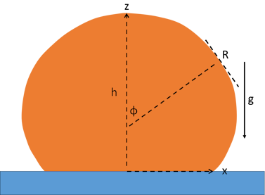
There are 3 interconnected equations governing the shape. They depend on b, h, σ, ρ and on g, gravity. Note that the contact angle, θ, doesn't appear as an input - discussed below. They relate to the angle φ which is 0 at the top of the drop and increases as you go downwards. The x-axis is horizontal and z is vertical. The radius of curvature at each point is R, with R=b at the lowest point. We then have:
- `(δx)/(δφ)=Rcosφ`
- `(δz)/(δφ)=Rsinφ`
- `1/R=(Δρg)/σ (h-z)+2/b-(sinφ)/x`
There is no analytical solution to this, so you just start at the bottom and step through small increments in φ. The numerics can explode when your settings don't match potential realities, so don't be alarmed by strange results.
The contact angle is simply φ when z = 0. Why are we deriving it from a complex equation rather than simply measuring it via a stanard method - such as fitting a spherical cap shape? The answer is that for very small drops, where the mass of the drop does not affect the shape, the spherical cap fit is fine. But larger (more practical) drops start to deform, needing the Y-L fitting. This means that the contact angle isn't the "true" angle. Whether it's possible to go from the Y-L fit to a "no gravity" value is something I don't yet know.
Thresholding, Lighting, Image Width
The technique for going from image to outline for you to fit is rudimentary - it depends on your threshold value. With a good image, even large changes to the threshold value will not alter the drop shape significantly. But with real-world images you may have to play around to get the best balance. The trick is to choose a threshold, measure θ, then change the threshold and re-measure θ. If it changes a lot then you probably need a better image. If the change is small, then you can be confident in the result. You will find that choosing the right box around the drop (via xMin etc.) many problems of thresholding will disappear.
There are sophisticated image analysis techniques which might make shape extraction more accurate in the case of poorer-quality images. But experience shows that there's no substitute for a good original image. So pour your energies into a setup that is at the same time simple and reliable.
Lighting is key. Modern "YouTuber" USB-chargeable diffuse LED lights are low cost and excellent. Artefacts from poor lighting get in the way of reliable thresholding. Anything in the path of the light will interfere with the contrast, as will up/down tilt in the platform. Reflections from the drop also make it harder to define the drop edges.
Defining the width is surprisingly simple. Cut out a piece of a ruler, say 5mm x 30mm, containing mm scale markings. Stick something to the back so you can place it on the platform at the same distance from the microscope lens as the droplet. You can easily read out the width to sufficient accuracy. If you have a fancy graticule with finer gradations, that's better, but the simple piece of ruler works well.
How accurate are the results?
You can answer this question yourself. Although there are many fancy techniques claiming to provide high accuracy, you can't do better than the quality of the setup (e.g. how level it is) and of the image (contrast, reflections, sharpness, focus, ...). By changing the relevant parameters over a modest range, you can see how much or little your calculated angle changes, and choose the best compromise as your final value.
Then you need to ask what accuracy you need. What outcomes depends on that angle? If ±1° makes little difference to the outcome, you're fine. If you worry about ±0.1° then you should use professional equipment.